Short Note on Corp (or Risky) Credit Term Structure

Bootstrapping the risk-free yield curve is (relatively) straightforward. One might be tempted to repeat the same trick for Corp bonds, i.e. bootstrapping a risky yield curve and use it for pricing by adding it to the risk free rate.

However, this approach would produce very poor results especially for lower rating bonds. If one starts from short maturity and move to longer maturities according to the naive scheme, the yield usually

• fluctuates a lot
• drops sharply (thus almost surely producing an inverted curve)
• or even unfolds in a way such that the PV of the earlier coupons of a long dated bond exceeds its observed price!

The problems arise because by adopting the naive bootstrapping approach that is borrowed from the risk free case, we completely ignored the effects of 1) recovery; and 2) CF timing shortening (due to default), which are dominant in the case of low rating bonds. Remember, the naive procedure is based on discounted (known) CF with no uncertainties either in timing or amount. When default is not only possible (since we are considering corp) but probable (since we are considering low ratings), this method breaks down.

One way to get by is to back out not the risky yield but the hazard rate (or equivalently the risk neutral default probability). To do that we have to express market bond price as a function of recovery and hazard rate, much like what is done for CDS pricing.

Reference:
Berd et al. 2004, "Defining, Estimating and Using Credit Term Structures" Part 1-3

Follow-up: Multi-curve Modeling

In [Mercurio 2009], two different approaches are proposed as attempts to resolve the new post-crisis market norm. (Recap: the issues include rate dependence on contract tenor, failure of textbook no-arb relationships between different rate securities)

The first approach focuses on the difference in counterparty risk for various contracts. For example, regarding the textbook case of replicating an FRA using a long and a short LIBOR deposits, we can introduce hazard rate and default time into the replication argument. That way, we end up with a forward LIBOR that is higher than the comparable FRA.

This approach, however, cannot be easily utilized in pricing, and more importantly the industry seems to favour 'segmenting market rates,' i.e. having multiple curves in existence simultaneously.

Digression: Bootstrapping
This is a description of how zero curve bootstrapping is done in general setting. (i.e. not limited to post-crisis multi-curve method)

A single kind of contract is unlikely to cover the entire range of maturities, hence different securities are required for different sections of the curve. What actually got to be chosen for curve construction depends on currency, but in general:

• The shortest end is built from cash/money market deposit. Since there is only a single bullet payment in a deposit transaction, the 'bootstrapping' is trivially done by day count (and perhaps compounding) adjustment.
• The middle section is built out of FRA or ED future contracts. Once again, since there is only one cash flow the bootstrapping is straight forward. Note however that if future contracts are used, a convexity adjustment is required so that the adjusted rate is comparable to that of a forward contract. (the convexity comes from the relative advantage of holding an interest rate future over forward, because MTM profit/loss can be reinvested/covered at a higher lower/rate)
• Finally, the far end of the curve is built out of swap. In this case we have to proceed in an order of ascending maturity because there are more than one payments in a swap. Suppose the rates are known up to (t-1). Then, with the market swap rate, S(t), and the discount factor up to (t-1), P(0,T_i), the discount factor and hence the rate for t can be found using the swap rate formula.

End of Digression

In the multi curve case, the only difference from the general procedure above is that we would only use one family of securities in building a curve of a certain tenor. (e.g. 3m deposit, 3m FRA with various maturities and 3m LIBOR fixing swaps with various number of payments to build the 3m tenor curve)

Finally, as an aside, note that curve interpolation is a tricky business, especially if you want to also calculate the instantaneous forward curve which is very sensitive to local curve fluctuations.

Multi-curve Pricing: Short Notes

Issue:
After Mid 2007, a lot of the good-o textbook wisdom failed to hold, mainly in two aspects:

1. Some rates use to match one another almost exactly (i.e. zero spread), for example deposit rate vs overnight swap rate; now the spread is much larger.
2. Swaps with different settlement frequencies have very large rate spread, i.e. the size of the swap rate depends on the fixing.

Proposed remedies:

1. Use separate curves for discounting and forwarding
2. Treat LIBOR's with different fixings as independent underlyings

Questions:
Even in the good-o textbook context, shall we expect LIBOR's with different tenors to have zero spread? Or is it just that tenor used to be irrelevant in the old narrative?

Reference:
Henrard 2009, "Irony in Discounting: The Crisis"
Bianchetti 2009, "Two Curves, One Price"
Mercurio 2009, "Interest Rates and the Credit Crunch: New Formulas and Market Models"

Credit Flattener and Steepener: Duration and Convexity Exposures

Flattener/Steepener are long/short strategies that bet on the relative movements of long vs. short maturity ends on a curve. The curve can be interest rate, variance or credit spread. For the sake of discussion, we consider a credit spread flattener.

The three main exposures are TIME, CURVE SHIFT and DEFAULT. Here we focus on CURVE SHIFT. Surely, we can mitigate the risk by duration hedging (even so we will be left with convexity risk, see below). However, notional matching has the advantage of zero default exposure (at least until the shorter leg expires).

In a notional-matched flattener, the investor speculate on flattening credit curve by selling (buying) CDS protection at the long (short) end. If the curve steepens instead, we would of course have a loss. What if the curve tightens by a parallel shift?

The mark-to-market as the spread moves is calculated by multiplying spread change to risky DV01, which, to recap, is the CDS spread numeraire. Obviously, DV01 of longer leg > DV01 of shorter leg. Hence a parallel upward shift (widening) of the curve affects the long leg more. But widening spread is bad for protection seller. Therefore a flattener position is harmed by widening spread (because the benefit on the short end < the loss on the long end).

The previous paragraph assumes that DV01 remains constant when the shift is small enough, and it considers only the relative sizes of DV01's. Not surprisingly, DV01 itself does not stay constant as the curve shifts further and hence there is convexity effect, which concerns the relative sensitivities of DV01's. Turns out DV01 decreases as spread widens, and the DV01 of the long end is more sensitive to curve shift than the short end. It follows then, that a flattener has positive convexity (when spread widens => DV01 drops => bad effect at long end diminishes => good for investor) while steepener has negative convexity.

Reference: JP Morgan 'Credit Derivatives Handbook'

Quick Notes on IR/Credit/Volatility Comparison

Modeling Approaches
Stochastic instantaneous spot
Short rate - Hazard rate - Stochastic volatility

Stochastic instantaneous forward
Instantaneous forward rate - ??? - xi in the Bergomi model

Market traded
LIBOR/Forward swap rate - Forward CDS rate - Forward variance swap rate

Others (Not exactly modeling)
Yield - ??? - Implied volatility

Question: where does local volatility fit in?

Great link on swap spread

http://fermatslastspreadsheet.wordpress.com/2012/01/11/facts-intuition-and-rules-of-thumb-for-swap-spreads/

Not just introduces the concept but also discusses how to put it in credit/rates trading context.

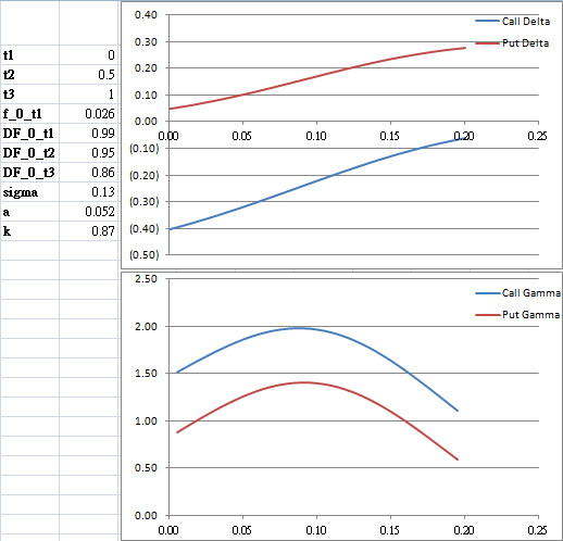
Short Rate Delta & Gamma (Hull-White One Factor)

Selection of European bond option greeks plots.

t2: option expiry

t3: underlying maturity

sigma: H-W volatility

a: H-W mean reversion

k: strike

x-axis: short rate

Pricing Callable Coupon Bond

Pricing a European callable zero-coupon bond is relatively straight forward. In fact, the callable zero-coupon bond can be decomposed into a non-callable zero-coupon bond and an European call option. Under many models (e.g. Hull-White), closed-form solution exists for European call option written on zero-coupon bond.

However, in reality, most callable corporate bonds bear coupons and the embedded options are American. In this case pricing would be much more complicated. First of all, since the embedded options are American, optimal exercise has to be considered. Secondly, the call on the principal plus the coupons cannot be seen as a basket of options because the option holder could only exercise the right to call everything, not an individual piece of cash flow.


There are at least 3 ways to tackle the pricing of callable coupon bonds:

1. Structural model - much like the structural credit models, we can postulate a model that describes how exercise strategy and hence option price are affected by the goal to minimize firm liabilities, by assuming a stochastic firm value process. Like other structural models, the drawback is that complete firm information is required.
2. Reduced form model (American option) - this is similar to the pricing of callable zero-coupon bonds, namely by explicitly considering the embedded call. The drawbacks are that a) the bond can never exceed par (the same problem arises in MBS reduced form pricing), and b) numerical method is necessary.
3. Reduced form model ("call intensity") - Jarrow et al proposes a method that treats the call feature as a hazard besides credit default risk. The approach is very similar to the reduced form model of Duffie and Singleton 1999. If the call intensity process is affine, closed-form solution exists.

Reference: Jarrow et al 2006, "Reduced-Form Valuation of Callable Corporate Bonds"

Negative duration of FRN

Floating Rate Note (FRN) usually has duration very close to zero. An FRN is reset to par on every reset date when the floating coupon is paid out. However it could have negative duration when it is traded at substantial discounts. Since, as we have already mentioned, the coupon of an FRN is floating, the discount is most probably due to credit instead of interest rate. Suppose then that an FRN is traded at a discount because of credit concern. Then we can write

FRN = FRN' + X

where FRN' is a note at a discount, FRN is an otherwise identical par note and X is some instrument that can be constructed so that the above expression holds. The point is that X has positive duration (as can be shown easily if we assume that the cash flow of FRN' is that of FRN with an extra spread S). Since the duration of FRN is close to zero, and the duration of X is positive, we must have that the duration of FRN' is negative.

(Possible) Quant Interview Questions

1. Maths
What is i^i? Give your answer to 2 decimal places for both the real and the imaginary parts.

2. Black-Scholes
Assume Black-Scholes and no dividend. P and C are, respectively, European vanilla put and call that are otherwise identical. What is the strike price that would make
i) their price; and
ii) their delta
the same?

3. Fixed income
The current yield curve is upward sloping. You speculate that it will get steeper and want to take advantage of it by long-shorting zero coupon bonds with different maturities (5 yrs and 10 yrs).
i) What is the duration-neutral strategy?
ii) What is the impact to your duration-neutral portfolio if there is a small parallel shift in the yield curve? A large (>>1bps) upward shift? A large (>>1bp) downward shift?

See here for more interview questions/brainteasers

Short note on ways to avoid negative short rate

- BK, BLT or other exponential-Gaussian models
- Imposing absorbing or reflecting BC (Goldstein and Keirstead)
- Kim and Singleton reviewed a few possibilities:

• Affine models like CIR, under which zero is not accessible
• Quadratic Gaussian models
• Black's shadow rate (i.e. treating bond yield as a call option to a latent process that CAN go negative)

MC Simulation for Hull-White Model

Recipe 1
Fit kappa and sigma by calibrating to swaptions/caps (swaption and cap prices can be expressed as Hull-White bond options, which in turn can be expressed as function of H-W bond price). Then calculate theta(t) by taking partial derivative of instantaneous forward rate f(0,t). Then do Euler MC simulation:

$r(t)=r(s)+(\theta (t) - \kappa r)dt + \sigma dW$

Recipe 2
This alternative method doesn't require taking partial on f(0,t). After fitting kappa and sigma,
then do the following MC simulation (it is by integrating the SDE):

$r(t)=r(s)e^{-\kappa (t-s)} + \alpha(t) - \alpha(s)e^{-\kappa(t-s)}+B$

where B is a Gaussian distributed white noise with variance

 $ \frac {\sigma^2}{2 \kappa} [1-e^{-2 \kappa (t-s)}]$

and

$\alpha(t) = f(0,t) + \frac {\sigma^2}{2\kappa^2}(1-e^{-\kappa t})^2$

Bottom line is, theta-fitting is about calibrating to the spot curve. But Recipe 2 does just that without invoking theta, because the instantaneous forward rate contains the same information.

Ref: Brigo pp.73

Also:
One can simulate the stochastic short rate process under the T-forward measure instead of the risk-neutral measure. The drift of the SDE will be different from that above, and would depend on T.

Advantage:
Since under the T-forward measure we discount the payoff with zero coupon bond, and the zero coupon bond price is completely determined by the short rate at a certain moment, we don't have to simulate too many points on a path, but we do need to do that for risk-neutral measure pricing in order to approximate the money-market account well.

Disadvantage:
P(t,T) bond is the natural numeraire to use for discounting, but what if we are pricing an instrument with multiple cash flows?

Shadow Rate

The original paper by Gorovoi and Linetsky, and a summary of it, is a pretty neat idea to resolve the shortcoming of Gaussian short rate models: that the interest rate can go below zero (but should we be concerned about negative rate, now that CHF Libor has seen negative values?).

The 'shadow rate,' which is a latent unobservable process, is still assumed to be Gaussian. The true short rate process is floored at zero of the latent process. Intuitively, people can always choose to hold cash when rate is below zero so the effective rate should never drop to negative.

They also use an eigenfunction expansion method to construct the solution to the PDE (derivative price).

The volatility of corp bond yield

Q: How does the volatility of the yield of corporate bond compare to that of treasuries?

A: The question can be translated into "is the correlation between corporate yield spread and the underlying index yield (treasury yield) positive or negative?" Empirical study shows that they are negatively correlated. What is the economic story? When the underlying riskless treasury yield is high, the general economy is usually doing well (i.e. what is the objective of the Fed?) and so the corporates are in good shape to service their debts. Default is therefore less likely.

Since the correlation is negative, the answer to the original question is that the yield of corporate bond actually tends to be lower than that of treasury securities. This is a little anti-intuitive, as we expect the corporate bond to be riskier and hence has more volatile price.

Instantaneous vs. Terminal volatility/correlation

Instantaneous vol. and correlation refer to the sigma and rho within the SDE's.

Terminal vol. and correlation require integrations. For an explanation on how instantaneous and terminal correlation differ, see Brigo pp.234-237.

Question to think about: are variance swap and correlation swap trading on instantaneous or terminal vol./correlation?

Trading Interview Questions

Brainteaser 1
There are N dice, each having x faces. What is the number of combination that give at least one 1 or x?
Ans: (x - 2)^N

Brainteaser 2
What is the longest diagonal within a k-dimensional hypercube?
Ans: sqrt(k)

Finance 1
You purchase a 5yr pure discount bond at 5% yield. One month later you sell it at 4% yield. What is the IRR of this investment?
Ans: ~60%

Finance 2
You enter into a pair trade consisting of CDS_A of 5yr tenor and 100bps, and CDS_B of 5yr tenor and 300bps. Suppose the spread narrows down to 100bps (from 200 bps) after 1 year and you are to unwind it. Describe the strategy and estimate the profit of this trade.
Ans: Sell protection with CDS_B and buy protection with CDS_A. Profit = 600bps (why?)

Finance 3
Part I
You, an American investor, are holding a 10yr convertible bond that is convertible over the first 5 years. Explain what risks you are exposed to and how they can be hedged away.
Ans:
a) Price risk (wrt the underlying equity). Can be hedged by shorting vanilla call.
b) IR risk. Can be hedged by shorting one (or more) zero coupon bonds, or entering into a fixed EUR for floating EUR swap.
c) FX risk. Can be hedged by entering into a floating EUR for floating USD swap.
NOTE: or we can enter into a fixed EUR for floating USD swap to hedge both IR and FX risks.
d) Credit risk. Can be hedged using CDS.
Part II
Suppose this is the only bond issued by the company. How do you calculate/estimate the price of a non-convertible 5yr bond issued by the same company?
Ans:
1. Strip away the embedded option to find the price of non-convertible 10yr
2. Find the spread of non-convertible 10yr over treasury curve/LIBOR swap curve
3. Here we have to make some sort of assumption regarding the term structure of the spread: constant, or usually slowing increasing
4. Using the spread term structure, find the spread of non-convertible 5yr over treasury curve/LIBOR swap curve
5. Using the spread of non-convertible 5yr over treasury curve/LIBOR swap curve, find the yield and hence the bond price

See here for more interview questions/brainteasers

LMM Calibration & Parameterization

Refer to Brigo Ch.6.

The 'calibration' of LMM to market data is trivial - since LMM is designed so as to be consistent with Black volatilities, the 'calibration' amounts to simply bootstrapping the caplet vol. from the cap vol.

However, we don't just want to use LMM to price caps/floors. We want to price other more exotic products. Hence we also have to specify the instantaneous volatilities (the diffusion coefficient sigma in the SDE) and the instantaneous correlations (the rho among the Brownian motions). Remember, if the payoff of an instrument depends on more than one LIBOR forward rates, then it depends on the terminal correlation, which in turn depends on both instantaneous volatility AND instantaneous correlation(Brigo pp.234). Note that we are assuming the scalar LIBOR specification (see here).

# LMM requires that sigma be deterministic. Hence parameterizing sigma amounts to choosing a deterministic function (of time) for the volatility term structure. Parameterizing sigma has nothing to do with fitting to market data.

# Meanwhile, correlation is a constant (matrix). By parameterizing the rho matrix we reduce the rank (i.e. degree of freedom) of the matrix. Parameterizing rho has nothing to do with fitting to market data.

Convexity, Time and Quanto Adjustments

Under the simplest B-S setting, the price of a forward contract does not depend on the volatility (cf. the price of a vanilla call). This makes sense because while the option payoff is asymmetric, hence would benefit from higher volatility, the forward payoff is symmetric (you lose money when the underlying price goes under water) and hence would neither benefit from nor be harmed by higher vol. However, in some cases the volatility comes into play even when the contract payoff is symmetric, and here we consider a few examples. The common theme of them is that we are trying to price an instrument under the "wrong" numeraire, which introduces an extra drift that does depend on the volatility.

Convexity/Time Adjustment
When the payoff is a linear function of the spot rate. The "wrong" numeraire is the zero coupon bond that does not expire on the right date (i.e. in-arrear swap or in-arrear cap/floor).

Quanto Adjustment
When the payoff is a linear function of the asset denominated in a foreign currency. The "wrong" numeraire is the domestic money-market account.

Reference:
Hull - Options, Futures and Other Derivatives [Chapter 29]
Veronesi - Fixed Income Securities [Section 21.7]
Brigo - Interest Rate Models [Chapter 13]

Fixed Income Mathmetics

LIBOR rate and Bond price
L(t,S,T) = -(p(t,T) - p(t,S))/((T-S) p(t,T))
* LIBOR is just discretely compounded forward rate

Continuously compounded forward rate and Bond price
R(t,S,T) = -(log(p(t,T)) - log(p(t,S)))/(T-S)


Instantaneous forward rate and Bond price
f(t,T) = -d(log(p(t,T)))/dT

Instantaneous short rate
r(t) = f(t,t)

Bond price and Instantaneous forward rate
p(t,T) = exp[-\int^T_t f(t,s) ds]
Note: this is just the inversion of the f vs. p formula above

Bond price and Instantaneous short rate
p(t,T) = E^Q[exp[-\int^T_t r(s) ds]]
Note: this comes from valuing a 1 dollar payoff under the Q-measure

Different Rates

- Federal Funds Rate
Bank lending Fed funds to other banks

- Prime Rate
Bank lending money to its customers

- Repo/Discount Rate
Fed lending its own money to banks
See: Discount Window

- LIBOR (London Interbank Offered Rate)
Bank lending money to other banks

- OIS (Overnight Indexed Swap)
Banks paying/receiving floating/fixed with other banks
Note: The swap rate is usually in between LIBOR and the Fed funds rate
See: OIS

- Eurodollar
Banks lending USD outside US

What does the LIBOR-OIS spread tell us?
Both LIBOR and OIS are between two risky counterparties, but OIS is less risky (because of swap payment and nominal amount netting). Hence the LIBOR-OIS spread is a measure of banks' credit risks.