So here is a game that recently came to mind. The two-player case is almost trivial, but let's begin with it anyway.
There are players A and B. The game is turn based, at the beginning of each turn they bet on the result of the turn: A wins or B wins (so a person is allowed to bet on herself), where win is defined as scoring more points than the other person. The scoring rules are:
1. An "A wins" bet gives one point to A; the same goes for B.
2. Betting on the right winner gives a point (i.e. if B bets that A wins and A does win, then B scores a point)
At the end of the turn, calculate the points. A "draw" is called if either logical contradiction is resulted, or the two players tie in score. When there is a draw, a new turn is played. As soon as there is a loser, the game ends. There are four scenarios:
1. A bets A wins; B bets B wins
2. A bets B wins; B bets A wins
3. Both bets are A wins
4. Both bets are B wins
Let's investigate the outcomes.
For scenario 1, each player gains one point, so it's a draw.
For scenario 2 also, each player gains one point, so it's a draw.
For scenario 3, A scores 3 points versus B scores 1 point, A wins.
For scenario 4, A scores 1 point versus B scores 3 points, B wins.
So assuming everyone wants to be the winner, the best strategy is to bet on oneself. Now we introduce a new rule to make the game more fun: one can bet against a certain player, i.e. bet that she loses:
1. An "A loses" bet deducts one point from A; the same goes for B.
2. Betting on the right loser gives a point (i.e. if B bets that A loses and A does lose, then B scores a point)
It seems that for a 2-player game, the new rules do not change the nature of the game much. Thus the best strategy is to bet on oneself (or, equivalently, to bet that the other person loses). What if there are three players? Would it still be the case that the best course of action is to always bet on oneself?
Wednesday, November 28, 2012
Tuesday, November 27, 2012
Those damn coins... (Part III)
This is the final episode of coin flipping problems (previous discussions can be found here and here). Last time we ended the discussion with the expected number of toss such that the sequence HH (or other combinations like HT or THH) appears for the first time. Now we consider playing games involving H and T combinations. The first type of game concerns the probability of combination A appearing before B does while flipping an unbiased coin.
CT08
Keep flipping a fair coin. What is the probability that the sequence HTT appears before HHT does?
CT08 - Answer:
This can be solved by setting up the problem as a Markov chain and calculating the absorption probabilities. Alternatively, letting A = HTT appears before HHT, we can consider the conditional probabilities conditioning on the first 3 flips:
P(A)
= P(A|HHH) + P(A|HHT) + P(A|HTH) + P(A|HTT) + P(A|THH) + P(A|THT) + P(A|TTH) + P(A|TTT)
Now it's time to simplify terms:
P(A|HHH) = 0
P(A|HHT) = 0
P(A|HTH) = P(A|H)
P(A|HTT) = 1
P(A|H) = P(A|T) = P(A)
So
P(A) = 1/8 * 0 + 1/8 * 0 + 1/8 * P(A) + 1/8 * 1 + 1/2 * P(A)
=> P(A)= 1/3
The second type of game is a little different from the previous case:
CT09
Two players take turn tossing a fair coin. When the sequence HT shows up for the first time, the person who flipped the T wins. What are the probabilities of winning for each player?
CT09 - Answer:
Once again conditional probability saves the day. Let A = First player wins,
P(A) = 0.5 * P(A|H) + 0.5 * P(A|T)
But P(A|T) = P(B) = 1 - P(A) (because "the second player becomes the first" if the first toss give a T)
Also, P(A|H) = 0.5 * P(A|HT) + 0.5 * P(A|HH) = 0.5 * 0 + 0.5 * (1 - P(A|H))
=> P(A|H) = 1/3
So
P(A) = 0.5 * 1/3 + 0.5 * (1 - P(A))
P(A) = 4/9
See here for more interview questions/brainteasers
Tuesday, November 6, 2012
Those damn coins... (Part II)
Last time we saw a number of coin-tossing related interview questions. In this post we look at two types of more advanced coin-related problems:
1) (possibly) unfair coins with odds drawn from a continuous distribution, and
2) games involving trying to obtain a specific sequence of Heads and Tails
1) Coins with odds drawn from a continuous distribution
If we cannot be sure about the odds of the coin, there would be another extra degree of randomness.
CT05
Suppose you have an unfair coin with P(Tail) = p, p is an unknown constant. What is the probability distribution of N, where N is the event: 'The first Head shows up at the N-th toss', and what is the expectation value of N?
CT05 - Answer:
The probability distribution is simply the Geometric Distribution p^(N-1) (1-p).
The expectation value of N is E[N] = 1/(1-p), which can be found by
E[N] = Sum_(i=1)^(inf) i*p^(i-1) (1-p)
Noting that
i*p^(i-1) = (d/dp)p^i
Using this and exchanging the order of summation and differentiation, we get
E[N] = 1/(1-p)
Meanwhile, if the odds of Head itself is drawn from a known distribution, then we can compute the desired expected values with integrals:
CT06
Suppose you have an unfair coin, with probability of a head p ~ uniform(0,1). What is the probability of getting 2 (or n) heads with 2 (or n) tosses?
CT06 - Answer:
If the coin is fair, then P(2 Heads) = 1/4. But now we would have to integrate
\int_0^1 p^n U(0,1) dp = 1/(n+1)
So for 2 tosses P(2 Heads) = 1/3.
Note that while for a fair coin with n tosses, the probabilites of obtaining {1,2,3,...,n} Heads are binomial coefficients, in this case the probabilites of obtaining {1,2,3,...,n} Heads are identical.
2) Games involving trying to obtain a specific sequence of Heads and Tails
This is yet another popular genre of interview questions, possibly because the questions can be varied easily (for example, by modifying the desired sequence of H and T). There are two sub-types: i) what is the probability that sequence A would show up before sequence B does? and ii) what is the probability that sequence A would be obtained during the first/second player's turn? (assuming that the two take turns) The two sub-types are to be solved in different ways. Let's start with the expected number of toss for obtaining a particular sequence.
CT07
Keep flipping a fair coin. What is the expected number of toss such that the sequence HH appears for the first time? What about HT and HHH?
CT07 - Answer:
One can take the most general coute and solve this as a Markov chain problem. For short sequences, especially for repeating sequences (i.e. HH, TT, HHH, etc.), writing down a recursive formula should be faster. Let N(A) be the expected number of toss to obtain the sequence A. Then
N(T) = N(H) = 2
N(HH) = N(H) + 0.5 * 1 + 0.5 * (1 + N(HH)) => N(HH) = 6
The recursive formula can be understood as the two possible outcomes upon obtaining the first H: either another H immediately, in which case the sequence HH is complete, or a T, in which case one has to start over from scratch, hence the N(HH) on the right hand side. It is not hard to prove by induction that, for B = k consecutive H,
N(B) = 2^(k+1) - 2
is a close-form solution. For general sequences, the recursive formula approach still works, though you would have to know the expected number of tosses for the sub-swquences. For instance:
N(HT) = N(H) + 0.5 * 1 + 0.5 * (1 + N(T))
N(HTH) = N(HT) + 0.5 * 1 + 0.5 * (1 + 0.5 * N(HTH))
N(HHT) = N(HH) + 0.5 * 1 + 0.5 * (1 + N(T))
What if we want to know the probability that sequence A would show up before sequence B does? We'll discuss that next time.
See here for more interview questions/brainteasers
Sunday, November 4, 2012
Quick Notes - Trading Ideas
- Momentum can be a result of nonlinearity/positive feedback due to algo trading: buy and sell orders induce more orders of their own kinds. Also, especially during market open, order regularities is a sign of algo in action. Can those be detected and exploited?
- Support and resistance levels, together with trading volume, provide useful insights. However, support and resistance levels (and similarly some other price patterns) are difficult to be quantified. Can neural network help?
- Support and resistance levels and volume data are more useful for securities that does not attract a lot of hedging investors (examples: commodities futures, mid cap stocks; counter-examples: ETF, some index futures).
Monday, October 15, 2012
Those damn coins...
Coin tossing (or coin flipping) is one of the popular settings for probability questions. It might be of interest to contrast coin tossing and dice rolling:
- Coin tossing follows a binomial distribution (which converges to Gaussian); die rolling follows a uniform distribution.
- Tossing m coins gives an expectation value of m/2; rolling an m-sided die gives an expectation value of (m+1)/2.
Because of the binomial distribution, coin tossing problems usually are more involved than dice rolling in terms of arithmetics. The most straight-forward kind of coin problems would simply ask you about the mean and variance of the number of Head or Tail:
CT01
What is the expected gain if you are paid $1 for each head in tossing 4 fair coins? What is the standard deviation?
CT01 - Answer:
Remember that in n binary trials with single success probability p, the mean is np and the variance is np(1-p). So the expected gain is $2 and the standard deviation is $1.
Sometimes the question is framed as a game:
CT02
What is the probability that the number of Heads is greater than or equals to 2 when tossing 4 coins?
CT02 - Answer:
The Pascal numbers for 4 trials are {1,4,6,4,1}. Hence the required probability is (6+4+1)/16 = 11/16.
Once the number of tossing becomes large, the Law of Large Number is handy.
CT03
What is the probability that there are more than 60 Heads out of tossing 100 coins?
CT03 - Answer:
The last thing you want to do is to calculate the binomial coefficients explicitly. Instead, observe that the probability distribution converges to a Gaussian as number of trials goes to infinity, with mean equals fifty and variance equals 25 (hence the standard deviation is 5). 60 is two standard deviations away from the mean, and the 68-95-997 rule gives (1 - 95%)/2 = 2.5%.
Another way to ask coin-tossing brainteeasers is to play with Bayesian statistics.
CT04
There are three coins, one with a H side and a T side (coin A); one with both sides being T (coin B); one with both sides being H (coin C).If you draw one among them at random and toss it to observe a Head, what is the conditional probability that coin C is picked?
CT04 - Answer:
This is a typical Bayesian inference question. Let X = [coin C is picked] and Y = [the toss gives an H], then
P(X|Y) = P(Y|X)*P(X)/P(Y) = 1 * (1/3) / (1/3*0 + 1/3*1/2 + 1/3*1) = 2/3
Hope you find this helpful. More to come!
See here for more interview questions/brainteasers
Sunday, October 14, 2012
All those interview questions and brainteasers...
It has been a while since this blog was created. It is intended to be a handy way to look up questions and brainteasers for interview preparation, although from time to time other relevant and interesting stuffs are also discussed.
I have recently once again been looking at a lot of the popular quant interview questions, and an idea comes to mind: perhaps it is worthwhile to re-do some posts in a more systemic manner? Instead of listing the questions and answers out, maybe a discussion of the brainteasers according to their solution technique would bring about more benefits?
It is with this spirit that I embark on this little project. In the following number of posts I would try to group different interview questions into categories and discuss them in more detail, especially how one should approach and attack them. You would find that all previous interview questions/brainteasers posts are now linked here; those posts would remain where they are, so you can think of this post as an overview or introduction.
Where to find more interview questions and brainteasers?
There are two popular printed books that are used extensively in interviews:
A Practical Guide To Quantitative Finance Interviews by Zhou, and
Heard on The Street: Quantitative Questions from Wall Street Job Interviews by Crack
Also, Frequently Asked Questions in Quantitative Finance by Wilmott has a relatively short section on brainteasers, although it is a compilation of materials available on his awesome website (see below). Quant Job Interview Questions And Answers by Joshi et al seems to be a good source too, though I have not read it myself.
Apart from printed books, there is an abundance of resource on the internet. The brainteaser section on the forum of Wilmott.com often has some original questions. Sites such as Braingle and Brainden are dedicated to brainteasers, although those might not be the ones that usually show up during interviews. For those looking for real challenges, wu :: forums should be able to keep you busy.
Finally, if you search the site Glassdoor for a particular company, there will be a bunch of questions that are submitted by those who have interviewed with the firm, with attempts to answer the questions (the quality of which can vary). If you can read Chinese, mitbbs.com has more questions that have actually been asked by interviewers (usually banks).
What should I expect?
Some brainteasers don't really require lengthy calculation. It takes a very specific 'Eureka' moment to be answered. It's fair to say that you won't know the answer if you haven't seen it before. And in case you wonder, yes, such questions do show up at interviews.
Otherwise, the majority of the questions does require calculation. When you are practising, don't just memorize the answer (that's obvious). Think about 1) why the answer is what it is; 2) whether there are alternative, shorter and sweeter ways to solve it; and 3) if the question could have been altered or extended. One thing that I find especially useful is to verify the answers using simulations. That not only assures you of correctness, but also gives you some intuition, as well as a handy way to play with different parameters and assumptinos.
So, here we go:
The series
Those damn coins...
Those damn coins... (Part II)
Those damn coins... (Part III)
More Coin Problems
Those damn dice...
Those damn dice... (Part II)
Those damn cards...
Friday, September 28, 2012
Brainteaser: What's my 10-digit number?
I'm thinking of a 10-digit number, where each digit represents the
number of that ordinal number in the whole number. So, the first digit
represents the number of 0's in the whole 10 digits. The second digit
represents the number of 1's in the whole 10 digits. And so on. The
first digit is not a '0.' What is my number?
Answer:
- Since the first digit is not zero, there is at least one zero among the digits.
- The sum of all digits must be 10 because it is a 10-digit number.
By some trials we find that the number 6210001000 fits the bill.
Follow-up question: is it the only correct answer?
See here for more interview questions/brainteasers
Wednesday, September 5, 2012
Timeline of Events Since 2007
The following is a non-exhaustive timeline of the events of the credit crisis:
2007 Dec - Fed's Term Auction Facility commenced.
2008 Mar - ECB extended the longest tender of Long Term Refinancing Operations (LTRO) to 6 months.
2008 Mar - Bear Stearns acquired by JP Morgan.
2008 Mar - Investment banks were allowed to borrow from the Fed's discount window.
2008 Jun - Countrywide Financial acquired by Bank of America.
2008 Jul - IndyMac placed into conservatorship.
2008 Sep - AIG bailed out by NY Fed.
2008 Sep - Goldman Sachs and Morgan Stanley became bank holding companies.
2008 Sep - Goldman Sachs bailed out by US government and Berkshire.
2008 Sep - Morgan Stanley bailed out by Mitsubishi UFJ
2008 Sep - Washington Mutual put on FDIC receivership.
2008 Sep - Lehman Brothers declared bankruptcy.
2008 Sep - Merrill Lynch acquired by Bank of America.
2008 Sep - Fannie Mae and Freddie Mac placed into conservatorship.
2008 Oct - Troubled Asset Relief Program (TARP) was signed into law.
2008 Oct - Wachovia merged with Wells Fargo.
2008 Nov - Quantitative Easing (QE) began. Fed started purchasing MBS securities.
2008 Nov - Citi bailed out by US government.
2009 Jan - Bank of England's Asset Purchase Facility (APF) began.
2009 Jun - General Motors filed for bankruptcy.
2010 Nov - QE2 began.
2011 Aug - US government downgraded by S&P.
2011 Sep - Fed announced Operation Twist.
2012 Sep - Fed announced QE3
2012 Sep - ECB announced Outright Monetary Transactions (OMT)
Tuesday, August 21, 2012
Book Review: Fooled by Randomness by Nassim Taleb
Spoiler Alert
I first came to know about Taleb years ago when I read his Dynamic Hedging. It was a great book with clarity and real-world wisdom that is rarely found in other option trading texts.
This book (and I believe the others of his), however, is completely different. I was hoping that despite the difference, Fooled by Randomness would still be tangentially related to option and trading, but the hope did not materialize. It is fair to say that the whole 300-or-so-paged book can be summarized as
I suppose these points are worth the discussion, although I would love to see them being explored at greater depth. And as mentioned eariler, you don't see much discussion in the context of derivative trading, which is a pity. Instead, too many sections are spent in recounting anecdotes and stories, ancient or modern, that may or may not be necessary.
All in all, the book is an easy read and I did get something out of it. Considering that Black Swan was published later than Fooled by Randomness and enjoys an inferior rating, I should pass on that and spend my time re-reading Dynamic Hedging instead.
http://www.amazon.com/Fooled-Randomness-Hidden-Chance-Markets/dp/1400067936/ref=sr_1_4?ie=UTF8&qid=1345545225&sr=8-4&keywords=taleb
I first came to know about Taleb years ago when I read his Dynamic Hedging. It was a great book with clarity and real-world wisdom that is rarely found in other option trading texts.
This book (and I believe the others of his), however, is completely different. I was hoping that despite the difference, Fooled by Randomness would still be tangentially related to option and trading, but the hope did not materialize. It is fair to say that the whole 300-or-so-paged book can be summarized as
- The signal-to-noise ratio of our media is low, if not zero;
- Trading and investing are perfect examples of fields containing a huge random component;
- A common problem among quants/financial economists is that they see market dynamics as something on which a descriptive/positive theory can be posited (think physics);
- Human mind is terribly bad at thinking in probabilisitc terms. In particular, emotions usually lead one into wrong conclusions/bad decisions.
I suppose these points are worth the discussion, although I would love to see them being explored at greater depth. And as mentioned eariler, you don't see much discussion in the context of derivative trading, which is a pity. Instead, too many sections are spent in recounting anecdotes and stories, ancient or modern, that may or may not be necessary.
All in all, the book is an easy read and I did get something out of it. Considering that Black Swan was published later than Fooled by Randomness and enjoys an inferior rating, I should pass on that and spend my time re-reading Dynamic Hedging instead.
http://www.amazon.com/Fooled-Randomness-Hidden-Chance-Markets/dp/1400067936/ref=sr_1_4?ie=UTF8&qid=1345545225&sr=8-4&keywords=taleb
Thursday, June 7, 2012
Book Review: Exotic Options Trading by Frans de Weert
I've been looking for a book like this one for a while. If you don't care for wordy review and just want to get a score, I'll hand it an 85/100, perhaps because I find this kind of book written by practitioners so rare (if you don't agree with that and instead have come across many of them better than this title, do leave a message below for me).
You would not find any fancy SDE or PDE in this book, though graphs are used to illustrate the option exposures and replications. When I said in the last paragraph that "this kind of book...[are] so rare" what I mean in particular is an in-depth analysis and explanation of concerns from a trader's perspective, e.g. what exposures would this exotic have, how to hedge it effectively, what are the execution risk when you are long/short, where does volatility skew come into play and so on.
Since the author was a trader he approaches the topic in a market-oriented fashion. For example, in the section discussing skew and smile the author explains how skew in FX market can be thought of in terms of the relative strength of the two currencies in the pair. The book is pretty well structured, starting with good-o option basics, Greeks, hedging, then goes on to volatility skew and smile, simple option strategies (call/put spread, straddle etc.) and finally to exotics.
The structure of the book is not too rigid, meaning that here and there the author would elaborate by inserting related discussions (the latter half is more formally structured, with each type of exotics constituting a chapter). This turns out to be a nice feature (well, to me at least) because it would really defeat the purpose if the "side" discussions were not intertwined into the "main" stuff. Plus, the book is not that long (200 pages) so this is more like a read-it-through text than your usual dictionary-sized desk top reference.
Pro:
- Quite clearly written
- Not many alternative titles with comparable scope/objective
Con:
- Doesn't discuss pricing and modeling (but then those are not the objectives of it, so not really a con)
- Occasionally some places seem to be not so rigorous. For example when using the put-call parity did the author forget to put in the cash term?
Bottom line:
Written by a trader for people who wants to learn more about real world concerns when trading options
p.s. Is book review like this helpful at all?
Saturday, June 2, 2012
Static Replication of Exotics
A number of exotics can be perfectly hedged by vanillas in a semi-static way (semi because unwinding is usually required when barriers are triggered).
P(K) stands for vanilla put option with strike K
C(K) stands for vanilla call option with strike K
BP(K) stands for binary put option with strike K
BDOT(K) stands for binary down one-touch option with strike K and postponed rebate R
The following assumes that spot equals forward equals zero.
Down-Out Call (H = K)
Initial hedge: charge S0-K premium and borrow K, buy a unit of stock
When barrier is hit: sell stock to receive K and pay back loan; option terminates worthless
If barrier never hit: sell stock to receive ST ; pay out max(S-K,0) and pay back loan
Note: in this case where H = K, there is no optionality.
Binary Up One-Touch with Rebate
The contract pays a fixed rebate R when stock price hits H from below before expiry.
Initial hedge: charge S0*R/H premium and use it to buy stock
When barrier is hit: sell stock to receive R and pay it out
If barrier never hit: sell stock and keep ST as profit
The following assumes that spot equals forward (for equity options this means interest rate = dividend yield).*
Binary Down One-Touch with Postponed Rebate
The hedge above is an overhedge in the sense that if the barrier is never breached, the writer gets to pocket the stock liquidation value at expiry. Here we try to more accurately hedge a contract that pays a fixed rebate R at expiry if stock price hits H from below before expiry.
Initial hedge: charge -R*P(H)/H+2*R*BP(H) premium to buy 2R units of binary put and sell R/H units of vanilla put with strike H
When barrier is hit: unwind to receive exp(-r(T-t))*R*[N(-d2)-N(-d1)], which, because S = H, equals exp(-r(T-t))*R. Put the amount into a money market account until expiry.
If barrier never hit: everything expires to give zero value
Down-In Call (H = K)
Initial hedge: charge P(H) premium and buy one put with strike H
When barrier is hit: sell put and buy call with strike H (self-financing by put-call parity)
Expires with barrier hit: pay out max(S-K,0), which is financed by the hedging call
If barrier never hit: put worthless; pays nothing out
Down-In Call (H > K)
Initial hedge: charge P(K)+(H-K)BDOT(H) premium to buy one put with strike K and (H-K) BDOT with strike H
When barrier is hit: sell put and BDOT to buy a call with strike K**
Expires with barrier hit: pay out max(S-K,0), which is financed by the hedging call
If barrier never hit: put and BDOT worthless; pays nothing out
Down-In Call (H < K)
Initial hedge: charge (K/H)*P(H^2/K) and buy (K/H) units of put with strike (H^2/K)
When barrier is hit: sell put and buy call with strike K (self-financing by put-call symmetry)
Expires with barrier hit: pay out max(S-K,0), which is financed by the hedging call
If barrier never hit: put worthless (it is OTM because the strike H^2/K < H and we know that stock never went below H); pays nothing out
* If this assumption is relaxed, we will have no perfect hedge but only upper and lower bounds. See reference.
** Sketch of proof: (first argument is stock price; second argument is strike)
When barrier is hit (S = H),
P(H,K)+(H-K)BDOT(H,H)
= P(H,K)+(H-K)[2BP(H,H)-P(H,H)/H]
= exp(-r(T-t))KN(...)-exp(-y(T-t))HN(...)+2exp(-r(T-t))HN(...)-2exp(-r(T-t))KN(...)
- exp(-r(T-t))HN(...)+exp(-y(T-t))HN(...)+exp(-r(T-t))KN(...)-exp(-y(T-t))KN(...)
= C(H,K)
Reference:
Gatheral "The Volatility Surface", Ch. 9
Bowie and Carr 1994 "Static Simplicity"
Monday, May 28, 2012
Variance Swap Revisited (Redux)
It's amazing how much I learn every time I re-read the variance swap literatures.
1. The (model-independent) formula for the fair strike of a variance swap depends on the choice of S* (the truncating spot price). Most generally it is
If S* is chosen to be the future stock price then the above expression can be simplified.
To hedge a variance swap, a trader statically holds the continuum of OTM options, plus rolling a future position of (1/F_t - 1/F_0). In a B-S universe the future position would hedge away the delta exposure, except that...
2. Delta of variance swap (one that comes from practicality):
In principal the terminal variance is measured as the INTEGRAL of INSTANTANEOUS variance; in practice, the contract is such that variance is calculated on a daily basis using daily prices. This leads to the need for intra-day Delta hedging.
3. Delta of variance swap (one that comes from smile)
The Coulombe paper show that variance swap Delta is a function of implied volatility skew. This implies that the Delta can be negative.
Reference:
Derman GS paper
de Weert "Exotic Options Trading" Ch. 23
Carr and Madan 2002 "Towards a Theory of Volatility Trading"
Coulombe et al 2008 "An Analytic Formula for the Delta of Variance Swap"
1. The (model-independent) formula for the fair strike of a variance swap depends on the choice of S* (the truncating spot price). Most generally it is
$ rT - \frac {S_0 e^{rT} - S^*} {S^*} - ln \frac {S^*}{S_0} + e^{rT} \int_0^{S^*} \frac {P(K)}{K^2} dK + e^{rT} \int_{S^*}^{\infty} \frac {C(K)}{K^2} dK$
If S* is chosen to be the future stock price then the above expression can be simplified.
To hedge a variance swap, a trader statically holds the continuum of OTM options, plus rolling a future position of (1/F_t - 1/F_0). In a B-S universe the future position would hedge away the delta exposure, except that...
2. Delta of variance swap (one that comes from practicality):
In principal the terminal variance is measured as the INTEGRAL of INSTANTANEOUS variance; in practice, the contract is such that variance is calculated on a daily basis using daily prices. This leads to the need for intra-day Delta hedging.
3. Delta of variance swap (one that comes from smile)
The Coulombe paper show that variance swap Delta is a function of implied volatility skew. This implies that the Delta can be negative.
Reference:
Derman GS paper
de Weert "Exotic Options Trading" Ch. 23
Carr and Madan 2002 "Towards a Theory of Volatility Trading"
Coulombe et al 2008 "An Analytic Formula for the Delta of Variance Swap"
Sunday, May 20, 2012
Short Notes on (Implied) Volatility
- At the risk of stating the obvious, implied volatility is nothing but the quoting of price under B-S framework. The use of it for anything else (i.e. hedging) is a recipe for disaster.
- In light of this, the purpose of having a stochastic volatility model is not primarily to have better fits to market smiles (though that is important too), but rather:
- To allow for consistent hedging (especially vega hedging);
- To prescribe some dynamics to the evolution of the smile^.
- In the B-S framework, if one long an option and continuously delta-hedge, the payoff would be 0.5*S*S*Gamma*(realized var. - implied var.)*dt. What about under a stochastic volatility model? Suppose that the variance process is also stochastic and we only delta hedge w.r.t. the stock price. If the variance process is dv = a dt + b dX, then the delta-hedged P&L would have a residual of b*Vv*dX, thanks to the additional source of randomness.
Reference: Rebonato, "Volatility and Correlation: The Perfect Hedger and the Fox" Ch. 6
Wilmott, "Paul Wilmott on Quantitative Finance" Ch. 12
Monday, May 7, 2012
Time Integral of Brownian Motion
This is a short note on computing the time integral of a Brownian motion:
$ \int_0^t W_s ds$
In fact I should have said the moments of such an integral. The first moment is just
$ E[\int_0^t W_s ds] = \int_0^t E[W_s] ds = 0$
The second moment is
\begin{align*} E[\int_0^t W_s ds \int_0^t W_u du] & = E[\int_0^t \int_0^t W_s W_u ds du] \\ &= \int_0^t \int_0^t E[W_s W_u] ds du \\ &= \int_0^t \int_0^t min(u,s) ds du \\ &= \int_0^t \int_0^s u du ds + \int_0^t \int_s^t s du ds \\ &=\int_0^t \frac {s^2} {2} ds+\int_0^t (ts-s^2) ds \\ &= \frac {t^3}{3}\end{align*}
\begin{align*} E[\int_0^t W_s ds \int_0^t W_u du] & = E[\int_0^t \int_0^t W_s W_u ds du] \\ &= \int_0^t \int_0^t E[W_s W_u] ds du \\ &= \int_0^t \int_0^t min(u,s) ds du \\ &= \int_0^t \int_0^s u du ds + \int_0^t \int_s^t s du ds \\ &=\int_0^t \frac {s^2} {2} ds+\int_0^t (ts-s^2) ds \\ &= \frac {t^3}{3}\end{align*}
The trick is to separate the min function into two
regimes.
Thursday, April 12, 2012
Short Note on Corp (or Risky) Credit Term Structure
Bootstrapping the risk-free yield curve is (relatively) straightforward. One might be tempted to repeat the same trick for Corp bonds, i.e. bootstrapping a risky yield curve and use it for pricing by adding it to the risk free rate.
However, this approach would produce very poor results especially for lower rating bonds. If one starts from short maturity and move to longer maturities according to the naive scheme, the yield usually
One way to get by is to back out not the risky yield but the hazard rate (or equivalently the risk neutral default probability). To do that we have to express market bond price as a function of recovery and hazard rate, much like what is done for CDS pricing.
Reference:
Berd et al. 2004, "Defining, Estimating and Using Credit Term Structures" Part 1-3
However, this approach would produce very poor results especially for lower rating bonds. If one starts from short maturity and move to longer maturities according to the naive scheme, the yield usually
- fluctuates a lot
- drops sharply (thus almost surely producing an inverted curve)
- or even unfolds in a way such that the PV of the earlier coupons of a long dated bond exceeds its observed price!
One way to get by is to back out not the risky yield but the hazard rate (or equivalently the risk neutral default probability). To do that we have to express market bond price as a function of recovery and hazard rate, much like what is done for CDS pricing.
Reference:
Berd et al. 2004, "Defining, Estimating and Using Credit Term Structures" Part 1-3
Monday, April 9, 2012
Quant Interview: High Frequency
1. What is CAPM?
2. If I have a portfolio of long option that are Delta hedged, what daily P&L can be expected?
3. If on average the probability of seeing one car passing by per hour is $\kappa$, what is the probability of seeing one car passing by within 15 minutes?
Ans: $1-(1- \kappa)^{1/4}$
4. How many integers fulfill all 3 criteria below:
See here for more interview questions/brainteasers
2. If I have a portfolio of long option that are Delta hedged, what daily P&L can be expected?
3. If on average the probability of seeing one car passing by per hour is $\kappa$, what is the probability of seeing one car passing by within 15 minutes?
Ans: $1-(1- \kappa)^{1/4}$
4. How many integers fulfill all 3 criteria below:
- 3-digited
- Odd
- Does not contain any '5' in any place
See here for more interview questions/brainteasers
Thursday, March 29, 2012
Follow-up: Multi-curve Modeling
In [Mercurio 2009], two different approaches are proposed as attempts to resolve the new post-crisis market norm. (Recap: the issues include rate dependence on contract tenor, failure of textbook no-arb relationships between different rate securities)
The first approach focuses on the difference in counterparty risk for various contracts. For example, regarding the textbook case of replicating an FRA using a long and a short LIBOR deposits, we can introduce hazard rate and default time into the replication argument. That way, we end up with a forward LIBOR that is higher than the comparable FRA.
This approach, however, cannot be easily utilized in pricing, and more importantly the industry seems to favour 'segmenting market rates,' i.e. having multiple curves in existence simultaneously.
Digression: Bootstrapping
This is a description of how zero curve bootstrapping is done in general setting. (i.e. not limited to post-crisis multi-curve method)
A single kind of contract is unlikely to cover the entire range of maturities, hence different securities are required for different sections of the curve. What actually got to be chosen for curve construction depends on currency, but in general:
In the multi curve case, the only difference from the general procedure above is that we would only use one family of securities in building a curve of a certain tenor. (e.g. 3m deposit, 3m FRA with various maturities and 3m LIBOR fixing swaps with various number of payments to build the 3m tenor curve)
Finally, as an aside, note that curve interpolation is a tricky business, especially if you want to also calculate the instantaneous forward curve which is very sensitive to local curve fluctuations.
The first approach focuses on the difference in counterparty risk for various contracts. For example, regarding the textbook case of replicating an FRA using a long and a short LIBOR deposits, we can introduce hazard rate and default time into the replication argument. That way, we end up with a forward LIBOR that is higher than the comparable FRA.
This approach, however, cannot be easily utilized in pricing, and more importantly the industry seems to favour 'segmenting market rates,' i.e. having multiple curves in existence simultaneously.
Digression: Bootstrapping
This is a description of how zero curve bootstrapping is done in general setting. (i.e. not limited to post-crisis multi-curve method)
A single kind of contract is unlikely to cover the entire range of maturities, hence different securities are required for different sections of the curve. What actually got to be chosen for curve construction depends on currency, but in general:
- The shortest end is built from cash/money market deposit. Since there is only a single bullet payment in a deposit transaction, the 'bootstrapping' is trivially done by day count (and perhaps compounding) adjustment.
- The middle section is built out of FRA or ED future contracts. Once again, since there is only one cash flow the bootstrapping is straight forward. Note however that if future contracts are used, a convexity adjustment is required so that the adjusted rate is comparable to that of a forward contract. (the convexity comes from the relative advantage of holding an interest rate future over forward, because MTM profit/loss can be reinvested/covered at a higher lower/rate)
- Finally, the far end of the curve is built out of swap. In this case we have to proceed in an order of ascending maturity because there are more than one payments in a swap. Suppose the rates are known up to (t-1). Then, with the market swap rate, S(t), and the discount factor up to (t-1), P(0,T_i), the discount factor and hence the rate for t can be found using the swap rate formula.
In the multi curve case, the only difference from the general procedure above is that we would only use one family of securities in building a curve of a certain tenor. (e.g. 3m deposit, 3m FRA with various maturities and 3m LIBOR fixing swaps with various number of payments to build the 3m tenor curve)
Finally, as an aside, note that curve interpolation is a tricky business, especially if you want to also calculate the instantaneous forward curve which is very sensitive to local curve fluctuations.
Wednesday, March 21, 2012
Multi-curve Pricing: Short Notes
Issue:
After Mid 2007, a lot of the good-o textbook wisdom failed to hold, mainly in two aspects:
Questions:
Even in the good-o textbook context, shall we expect LIBOR's with different tenors to have zero spread? Or is it just that tenor used to be irrelevant in the old narrative?
Reference:
Henrard 2009, "Irony in Discounting: The Crisis"
Bianchetti 2009, "Two Curves, One Price"
Mercurio 2009, "Interest Rates and the Credit Crunch: New Formulas and Market Models"
After Mid 2007, a lot of the good-o textbook wisdom failed to hold, mainly in two aspects:
- Some rates use to match one another almost exactly (i.e. zero spread), for example deposit rate vs overnight swap rate; now the spread is much larger.
- Swaps with different settlement frequencies have very large rate spread, i.e. the size of the swap rate depends on the fixing.
- Use separate curves for discounting and forwarding
- Treat LIBOR's with different fixings as independent underlyings
Questions:
Even in the good-o textbook context, shall we expect LIBOR's with different tenors to have zero spread? Or is it just that tenor used to be irrelevant in the old narrative?
Reference:
Henrard 2009, "Irony in Discounting: The Crisis"
Bianchetti 2009, "Two Curves, One Price"
Mercurio 2009, "Interest Rates and the Credit Crunch: New Formulas and Market Models"
Monday, March 5, 2012
Credit Flattener and Steepener: Duration and Convexity Exposures
Flattener/Steepener are long/short strategies that bet on the relative movements of long vs. short maturity ends on a curve. The curve can be interest rate, variance or credit spread. For the sake of discussion, we consider a credit spread flattener.
The three main exposures are TIME, CURVE SHIFT and DEFAULT. Here we focus on CURVE SHIFT. Surely, we can mitigate the risk by duration hedging (even so we will be left with convexity risk, see below). However, notional matching has the advantage of zero default exposure (at least until the shorter leg expires).
In a notional-matched flattener, the investor speculate on flattening credit curve by selling (buying) CDS protection at the long (short) end. If the curve steepens instead, we would of course have a loss. What if the curve tightens by a parallel shift?
The mark-to-market as the spread moves is calculated by multiplying spread change to risky DV01, which, to recap, is the CDS spread numeraire. Obviously, DV01 of longer leg > DV01 of shorter leg. Hence a parallel upward shift (widening) of the curve affects the long leg more. But widening spread is bad for protection seller. Therefore a flattener position is harmed by widening spread (because the benefit on the short end < the loss on the long end).
The previous paragraph assumes that DV01 remains constant when the shift is small enough, and it considers only the relative sizes of DV01's. Not surprisingly, DV01 itself does not stay constant as the curve shifts further and hence there is convexity effect, which concerns the relative sensitivities of DV01's. Turns out DV01 decreases as spread widens, and the DV01 of the long end is more sensitive to curve shift than the short end. It follows then, that a flattener has positive convexity (when spread widens => DV01 drops => bad effect at long end diminishes => good for investor) while steepener has negative convexity.
Reference: JP Morgan 'Credit Derivatives Handbook'
Tuesday, February 28, 2012
Quick Notes on Haug's Article (Know Your Weapon I)
Concerning vanilla options and good-O' Black- Scholes:
- Delta (the absolute value of which) can be greater than unity
- As a corollary, ITM put can have absolute Delta lower than 0.5 and OTM call can have Delta greater than 0.5
- Gamma and Vega attain their max NOT at-the-money-forward
- Ordinary way of computing Gamma has a saddle point; there's a peak at the long expiry zero underlying boundary
- As a consequence, GammaP might be more useful than Gamma in describing gamma risk
Saturday, February 11, 2012
Black-Scholes Pricing in F#
First, get Math.NET Library (Open source).
F# code:
\\ begin
#light
open MathNet.Numerics.FSharp
open MathNet.Numerics.Distributions
let d12 (S0,r,y,sigma,K,T,d1_d2) = (log (S0/K)+(r-y+(if d1_d2 = 1.0 then 1.0 else -1.0))*(sigma*sigma / 2.0)*(T))/(sigma * (sqrt(T)))
let normal = new Normal(0.0, 1.0)
let bsPrice (S0, r, y, sigma, K, T) = exp (-y*T) * S0 * normal.CumulativeDistribution(d12 (S0,r,y,sigma,K,T,1.0))-exp (-r*T) *K * normal.CumulativeDistribution(d12 (S0,r,y,sigma,K,T,2.0))
printfn "Price = %F" (bsPrice (1.0, 0.0, 0.0, 0.2, 1.0, 1.0))
open System
Console.ReadKey(true)
\\ end
Friday, February 10, 2012
Vega hedging (and good modeling practice in general)
Recently re-read two very good papers (see the bottom), and it's interesting to find that they have related themes.
Synopsis for Jarrow: A model can either be theoretical or statistical (think regression). A theoretical model can be rejected (or not) by inspecting the assumptions and implications (note, though, that a rejected model can still be used). If a theoretical model is rejected, then calibration to market data would effectively turn it into an ad hoc statistical model.
For the sake of discussion consider B-S. It sets out to be a theoretical model, but volatility smile renders it rejected. By calibrating it to the volatility smile (local volatility), we are turning it into a statistical model. It can then be used to price other options (although, now being a statistical model, the econometric relationship would change over time and re-calibration is required). What we should not do is to use it for Delta/Gamma hedging, because it is exactly the failure of Delta hedging assumption that breaks its theoretical model status - there exist more than one sources of risk, which is why a single constant sigma does not suffice.
What is worse than using it for Delta hedging is to use it for Vega hedging, because under B-S the stock volatility is assumed to be a constant. Taking partial derivative with respect to sigma is mathematically sound, but it makes no sense other than spitting out an expression that lure you into believing its legitimacy. Which brings us to the uncertain parameters model Wilmott discussed. In his paper (and his book too) he explains why Vega is a terrible measure of volatility sensitivity when Gamma changes sign. Besides cliquet option, barrier option also falls into this category.
He proposes an uncertain parameter model that still uses Delta hedging argument. A non-linear PDE is produced. In a related chapter he discusses a similar technique for interest rate modeling, although in that case Delta hedging is dropped and the result of calibration is a yield envelop.
Jarrow 2011 - Risk Management Models: Construction, Testing, Usage
Wilmott - Cliquet Option Pricing
Also, PWOQF Ch. 52
Tuesday, February 7, 2012
Quick Notes on IR/Credit/Volatility Comparison
Modeling Approaches
Stochastic instantaneous spot
Short rate - Hazard rate - Stochastic volatility
Stochastic instantaneous forward
Instantaneous forward rate - ??? - xi in the Bergomi model
Market traded
LIBOR/Forward swap rate - Forward CDS rate - Forward variance swap rate
Others (Not exactly modeling)
Yield - ??? - Implied volatility
Question: where does local volatility fit in?
Saturday, January 14, 2012
Stochastic Volatility One-Period Tree
We have three securities (money market account, stock, call option on the stock with K = 100). Today their prices are [100, 100, 8]. Suppose one period from now the stock can end up being either in the high-volatility (in which case S = 120 or 80) or low-volatility (in which case S = 110 or 90) regime.The MMA would still be 100. Now consider an exotic option X. The payoff of X is (30, 0, 0, 15) corresponding to (high vol stock up, high vol stock down, low vol stock up, low vol stock down). You can imagine it as a derivative that becomes a call when volatility is high and a put otherwise. What is today's value of X?
Ans: $12
Note: This problem is solvable because the matrix that represents basis securities payoffs has a left inverse. When would this be not true? -> When some basis security is the linear combination of others.
Ans: $12
Note: This problem is solvable because the matrix that represents basis securities payoffs has a left inverse. When would this be not true? -> When some basis security is the linear combination of others.
Thursday, January 12, 2012
Great link on swap spread
http://fermatslastspreadsheet.wordpress.com/2012/01/11/facts-intuition-and-rules-of-thumb-for-swap-spreads/
Not just introduces the concept but also discusses how to put it in credit/rates trading context.
Not just introduces the concept but also discusses how to put it in credit/rates trading context.
Tuesday, January 3, 2012
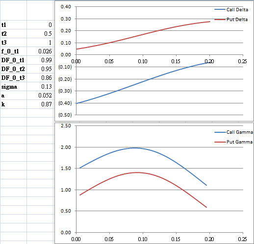
Short Rate Delta & Gamma (Hull-White One Factor)
Selection of European bond option greeks plots.
t2: option expiry
t3: underlying maturity
sigma: H-W volatility
a: H-W mean reversion
k: strike
x-axis: short rate


Pricing Callable Coupon Bond
Pricing a European callable zero-coupon bond is relatively straight forward. In fact, the callable zero-coupon bond can be decomposed into a non-callable zero-coupon bond and an European call option. Under many models (e.g. Hull-White), closed-form solution exists for European call option written on zero-coupon bond.
However, in reality, most callable corporate bonds bear coupons and the embedded options are American. In this case pricing would be much more complicated. First of all, since the embedded options are American, optimal exercise has to be considered. Secondly, the call on the principal plus the coupons cannot be seen as a basket of options because the option holder could only exercise the right to call everything, not an individual piece of cash flow.
There are at least 3 ways to tackle the pricing of callable coupon bonds:
- Structural model - much like the structural credit models, we can postulate a model that describes how exercise strategy and hence option price are affected by the goal to minimize firm liabilities, by assuming a stochastic firm value process. Like other structural models, the drawback is that complete firm information is required.
- Reduced form model (American option) - this is similar to the pricing of callable zero-coupon bonds, namely by explicitly considering the embedded call. The drawbacks are that a) the bond can never exceed par (the same problem arises in MBS reduced form pricing), and b) numerical method is necessary.
- Reduced form model ("call intensity") - Jarrow et al proposes a method that treats the call feature as a hazard besides credit default risk. The approach is very similar to the reduced form model of Duffie and Singleton 1999. If the call intensity process is affine, closed-form solution exists.
Subscribe to:
Comments (Atom)