This is by no means an attempt to promote high frequency trading (HFT). In fact, the HFT scene has become so crowded that even real pro shops are having a hard time, let alone retail traders with their home brew system (By the way, here is an interesting read. Judge for yourself how much to believe). So why should a trader trade more?
Because it's about how confident you can be in making a conclusion. If you make one trade in your life and it turns out winning, your rate of winning is 100% and yet the only legitimate conclusion you can make is...well, that you don't have enough data point. In the spirit of Bayesian statistics as was used here, we can formulate a simple analysis that hopefully would provide some insights.
Suppose that you are a manager about to hire a new trader for your team. There are two candidates, Andrew Flook who had 5 winning trades out of 5 last year; and Bob Luckson who had 70 winning trades out of 100 last year. Who should get the job? Since Andrew has a 100% winning rate and Bob has only 70%...are we missing something?
Let's cast this in the light of Bayesian statistics. Of course I would have to make some assumptions:
Winning probability of a fluke trader = p = 0.5
Winning probability of a skilled trader = q = 0.7
Total number of winning trades = W
Total number of losing trades = L
Unconditional probability that any trader is a skilled one = s = 0.2
The last assumption about a trader being a skilled one is based on the anecdotal evidence that only about 20% of all traders are profitable in the long run. So, if $R$ stands for the trading Results of last year, $S$($F$) stands for the trader being a Skilled(Fluke) one, we have
$$ P(R|S)P(S) = q^W (1-q)^L s $$
$$ P(R|F)P(F) = p^W (1-p)^L (1-s) $$
$$ P(S|R) = \frac {P(R|S)P(S) }{P(R|S)P(S) +P(R|F)P(F) } $$
Plugging in the numbers, we find that Andrew (the 100% guy) has a 57% chance of being a skilled trader, while Bob enjoys a 99.9% chance.
Friday, December 13, 2013
Saturday, November 23, 2013
How do you model the dynamics of asset prices? A self-reflection (2 of 3)
Last time we have set a stage for the discussion on modeling the dynamics of asset prices. Gaussian process is the "canonical" way to go, and we've seen the characteristics/limitations of it. To recap:
Candidate: Brownian motion
Poisson
We've already met Gauss last time. Now we'll introduce a contemporary of him, Siméon Denis Poisson. While Brownian motion is a diffusion stochastic process (a random walk down the street), the Poisson process is a counting process that is associated with jumps. When we add a Poisson counting process to the diffusion equation, the stochastic differential equation becomes a jump-diffusion equation that allows for jumps, or "gapping up/down". Why is this desirable or required? Just talk to any trader, and they'll tell you that price jump is a reality, especially for markets with substantial close hours (i.e. the majority of the markets other than FX, S&P futures...). So instead of a random walk down the street, perhaps after all it is more like parkour down the street?
You Jump, I Jump
What are the advantages of modeling asset prices with a jump-diffusion process over a diffusion only process?
Candidate: Jump-diffusion Process
The implementation of jump-diffusion model can be challenging. The numerical calibration is of course more computationally intensive, but the more subtle and fundamental issue is this: how do we identify jumps? When there is a "sudden" gap in the time series, how can one be sure that it is NOT just an extreme value, yet still being drawn from the good old Gaussian distribution?
Candidate: Brownian motion
- Markovian
- "Tractable"(-ish, depending on how you transform it)
- Excess kurtosis = 0
- Market completeness (if number of hedging instruments >= number of sources of randomness)
Poisson
We've already met Gauss last time. Now we'll introduce a contemporary of him, Siméon Denis Poisson. While Brownian motion is a diffusion stochastic process (a random walk down the street), the Poisson process is a counting process that is associated with jumps. When we add a Poisson counting process to the diffusion equation, the stochastic differential equation becomes a jump-diffusion equation that allows for jumps, or "gapping up/down". Why is this desirable or required? Just talk to any trader, and they'll tell you that price jump is a reality, especially for markets with substantial close hours (i.e. the majority of the markets other than FX, S&P futures...). So instead of a random walk down the street, perhaps after all it is more like parkour down the street?
You Jump, I Jump
What are the advantages of modeling asset prices with a jump-diffusion process over a diffusion only process?
Candidate: Jump-diffusion Process
- Markovian
- Not tractable (unless under restrictive assumptions)
- Excess kurtosis > 0
- Market incomplete (unless under restrictive assumptions)
The implementation of jump-diffusion model can be challenging. The numerical calibration is of course more computationally intensive, but the more subtle and fundamental issue is this: how do we identify jumps? When there is a "sudden" gap in the time series, how can one be sure that it is NOT just an extreme value, yet still being drawn from the good old Gaussian distribution?
Friday, November 22, 2013
Monty Hall, extended
The original Monty Hall problem is so famous that pretty much every soul knows the solution by heart (in case you don't: change to the other still closed door and double your winning probability!). Despite (or because of) the fame of this problem, some would learn the answer without really knowing how to solve it. Let's go through the problem in its original setting:
Classic Three Door Monty Hall
There are three doors A, B and C, and only one leads to a prize. After you picked door A, the host (who knows where the prize is) opens door C, which turns out to be not the prize door. What is the winning probabilities of you sticking to door A versus switching to door B?
And of course, the toolkit to invoke is Bayesian statistics:
$$ P(A|C_o) = \frac { P(C_o|A)P(A)}{P(C_o)} $$
where $P(X)$ is the unconditional probability of the prize being behind door X, and $P(Y_o)$ is the probability of door Y being opened by the host. In this case, the entities on the RHS are straightforward, except perhaps for $ P(C_o)$:
$$ P(C_o|A) = 1/2 $$
$$ P(A) = 1/3 $$
$$ P(C_o) = P(C_o|A)P(A) + P(C_o|B)P(B) + P(C_o|C)P(C) $$
$$= \frac 1 2 \times \frac 1 3 + 1 \times \frac 1 3 + 0 = \frac 1 2$$
So $P(A|C_o) = 1/3$. One can in a similar fashion find that $P(B|C_o) = 2/3$. The reason $ P(C_o|B) = 1$ is of course that if the prize is really behind door B, the host has no choice but to open door C.
Extended Five Door Monty Hall
So far so good. Now we are invited to a "Monty Hall Deluxe" game with a bigger prize, but more doors and more rounds. In round one, you pick a door. The host would open one door, after which you may choose to switch to another. Then once you have decided and acted accordingly, we enter round two where the host would open one more door (so number of closed door drops to 3 at this point). Then you decide on whether to switch for a second time, and if so to which door. What should the optimal strategy be?
Suppose you first pick door A and the host opens door E. The first round of this game is really similar to the Classic version above. Namely,
$$ P(A|E_o) = \frac { P(E_o|A)P(A)}{P(E_o)} $$
with
$$ P(E_o|A) = 1/4$$
$$ P(A) = 1/5$$
$$ P(E_o) =\sum P(E_o|X)P(X) $$
$$= \frac 1 4 \times \frac 1 5 + \frac 1 3 \times \frac 1 5 + \frac 1 3 \times \frac 1 5+ \frac 1 3 \times \frac 1 5+0 = \frac 1 4$$
So $P(A|E_o) = 3/15$. Similarly, one can show that $P(B|E_o) = P(C|E_o) =P(D|E_o) =4/15$. So once again, it is better for you to switch (and due to symmetry, it doesn't matter to which).
Suppose you switch to door B. Now we are in round two. The host then open door D, which, surprise-surprise, turns out to have no prize behind it too. Now what do you do? What are the probabilities of staying versus switching?
One thing to be careful about is this: since at this point round one is already over, the conditional probabilities we calculated (i.e. $P(A|E_o)$, $P(B|E_o)$, ...) should now be considered unconditional:
$$ P(A) = 3/15$$
$$ P(B) = 4/15$$
$$ P(C) = 4/15$$
We also have the followings:
$$ P(D_o|A) = 1/2$$
$$ P(D_o|B) = 1/3$$
$$ P(D_o|C) = 1/2$$
$$ P(D_o) =\sum P(D_o|X)P(X) $$
$$= \frac 1 2 \times \frac 3 {15} + \frac 1 3 \times \frac 4 {15} + \frac 1 2 \times \frac 4 {15} +0 = \frac {29} {90}$$
Hence $P(A|D_o) = 9/29$, $P(B|D_o) = 8/29$ and $P(C|D_o) = 12/29$. So staying with door B is even worse than switching back to door A, and switching to the untouched door C is the best. Just keep switching!
Sunday, November 17, 2013
How do you model the dynamics of asset prices? A self-reflection (1 of 3)
Having been working on/studying mathematical finance for a while now, I feel like it would be useful to step back and look at one of the most important topics in this area: how does one model asset price dynamics?
Gauß
The canonical account would inevitably begin with Gauss. The Gaussian distribution (or the normal distribution, depending on your academic upbringing) is undeniable the most well-investigated probability distribution in human history. We don't need to go into all the details and properties of it, but it's good to be reminded of a number of facts regarding how the normal distribution is related to some other entities:
Our Checklist
Before proceeding further, let's compile a checklist that we will re-visit multiple times in this series:
Candidate: Brownian motion
Gauß
The canonical account would inevitably begin with Gauss. The Gaussian distribution (or the normal distribution, depending on your academic upbringing) is undeniable the most well-investigated probability distribution in human history. We don't need to go into all the details and properties of it, but it's good to be reminded of a number of facts regarding how the normal distribution is related to some other entities:
- It is closely related to the phenomenon of diffusion;
- The Central Limit Theorem says that (under some technical conditions) the sum of many i.i.d. random variables would converge to a normal distribution;
- Brownian motion is mathematically described by Wiener process, which follows a Gaussian distribution.
Our Checklist
Before proceeding further, let's compile a checklist that we will re-visit multiple times in this series:
Candidate: Brownian motion
- Markovian
- "Tractable"(-ish, depending on how you transform it)
- Excess kurtosis = 0
- Market completeness (if number of hedging instruments >= number of sources of randomness)
- A Markov process has no memory. It doesn't matter if the market went up 20%, up 3%, down 3%, or down 20% yesterday. Today's probability of movement is not affected in any way.
- "Tractable" refers to a closed-form expression for the asset price process itself, or the price of derivatives with the asset as underlying.
- Excess kurtosis is a measure of "tail effect"
- Market completeness means a contingent claim can be fully hedged
Thursday, November 7, 2013
The Balanced 1-0 Matrix Problem
This post is about the Balanced 1-0 Matrix problem. Namely, for an n-by-n matrix (can be relaxed to n-by-m, but we will stick to square matrix here), how many legitimate assignments are there such that each row as well as column contains exactly n/2 zeros and n/2 ones?
You will find different approaches to solve this problem in the link, and one thing to note is how quickly the sequence grows: the numbers of possible assignments are 1, 2, 90, 297200... for 1-by-1, 2-by-2, 3-by-3, 4-by-4 matrices. The brute force approach is not very interesting, so we will only discuss the dynamic programming approach. The Matlab script can be found at the end.
The idea is first to have an easy way to store the arrangement. That is what stateArr does. As a 2-by-n array, it stores how many zeros and ones are still available to be allocated for each of the n columns. Then we have the systematic sweeping through the rows, meaning that we do a tree search starting from the first row downward. We iterate all the possible combinations (of course, they have to have n/2 zeros and n/2 ones) for a row, and compare these possible combinations against the stateArr to see if there are enough zeros and ones to be assigned. This is what the for loop within the DP_recursion is for.
Finally, the algorithm described above would have to visit every and all solutions unless we use a memoization trick. All partial solutions, as well as the corresponding stateArr, are stored in stateArrTable, and for every step the script would first check whether partial solution already exists. If so, use the stateArr as a signature/key to retrieve it; if not, and only if not, will it jump into recursion.
Unfortunately, even with dynamic programming, the computation is too intensive for Matlab for any n > 4.
function output = ZeroOneMat_DP(numCol)
% ((1, 2) (2, 1) (1, 2) (2, 1)) would be stored as
% [1, 2, 1, 2; 2, 1, 2, 1]
% First row is # zeros, second row is # ones
stateArr = numCol/2*ones(2,numCol);
stateArrTable = [];
partialAnsArr = [];
[output stateArrTable partialAnsArr] = DP_recursion(numCol, stateArr, stateArrTable, partialAnsArr, 0);
end
%%%%%%%%%%%%%%%%%%%%%%%%%%%%%%%%%%%%%%%%%%
function [output stateArrTable partialAnsArr] = DP_recursion(numCol, stateArr, stateArrTable, partialAnsArr, numSol)
% Iterate all combinations
locationMat = nchoosek(1:numCol,numCol/2);
tempOutput = numSol;
for i = 1:size(locationMat,1)
thisRow = zeros(1,numCol);
thisRow(locationMat(i,:)) = 1;
% Change stateArr
stateArr_temp = stateArr;
for j = 1:numCol
if thisRow(j) == 0
stateArr_temp(1,j) = stateArr_temp(1,j) - 1;
elseif thisRow(j) == 1
stateArr_temp(2,j) = stateArr_temp(2,j) - 1;
end
end
% Check if there is negative values
if min(min(stateArr_temp)) < 0
elseif min(min(stateArr_temp)) >= 0 & max(max(stateArr_temp)) > 0
% See if already in table
[foundBool theAnswer] = findInTable(stateArr_temp, stateArrTable, partialAnsArr);
if foundBool == 0 % not
[tempOutput2 stateArrTable partialAnsArr] = DP_recursion(numCol, stateArr_temp, stateArrTable, partialAnsArr, tempOutput);
% Save to partial answers
stateArrTable = [stateArrTable; stateArr_temp];
partialAnsArr = [partialAnsArr; tempOutput2 - tempOutput];
tempOutput = tempOutput2;
elseif foundBool == 1
% find in table
tempOutput = tempOutput + theAnswer;
end
elseif max(max(abs(stateArr_temp))) == 0 % successfully placed all numbers through the last row
tempOutput = tempOutput + 1;
end
end
output = tempOutput;
end
function [foundBool theAnswer] = findInTable(stateArr, stateArrTable, partialAnsArr)
foundBool = 0;
theAnswer = -1;
for i = 1:size(stateArrTable,1)/2
if max(max(abs(stateArrTable(2*i-1:2*i,:)-stateArr))) == 0
theAnswer = partialAnsArr(i);
foundBool = 1;
break
end
end
end
Tuesday, November 5, 2013
Those damn cards...
We are quickly approaching the end of the combo interview question bank series. So far we have discussed a variety of coin and dice problems. Yet another popular theme would be card games, specifically with poker decks. As compared to coins and dice, a poker deck contains two colours and four suits, giving rise to some interesting and complicated games and problems.
CF01
A deck consists of 3 red and 3 black cards. They are turned over one by one, and at any point you can make the call of the following card being red. If it turns out to be the case, you win. What is the optimal strategy?
CF01- Answer:
This is closely related to option pricing with binomial tree. Being able to call 'red' as you wish is equivalent to early exercise. It's trivial to show that without early exercise, the probability tree reads:
0.5000
0.3125 0.6875
0.1250 0.5000 0.8750
0.0000 0.2500 0.7500 1.0000
0.0000 0.5000 1.0000
1.0000 0.0000
corresponding to #Black card shown : #Red card shown
0:0
0:1 1:0
0:2 1:1 2:0
0:3 1:2 2:1 3:0
1:3 2:2 3:1
2:3 3:2
Remember, this is when there is no early exercise, meaning that you can only passively look at cards being flipped open and wait to see if the last card is red. To take early exercise into account, some nodes on the probability tree will be over-ridden, depending on the numbers of remaining cards on the node. Take the (1:2) node as an example. When 1 Black card and 2 Red cards are already shown, there are 2 Black cards and 1 Red card remaining in the deck. Hence the winning probability of early calling at this point is 1/3 = 0.333..., which is greater than 0.25. Hence the optimal strategy would require early calling at this node. Similar argument can be made regarding other nodes on the tree.
CF02
You draw a card from a deck and player B draws another. You win only if your draw has a higher number. What is the probability that you will win?
CF02- Answer:
P(numbers equal) = 3/51 = 1/17. Due to symmetry, the two parties have the same winning probability. Hence P(you win) = (1 - 1/17) / 2 = 8/17
See here for more interview questions/brainteasers
Wednesday, October 30, 2013
Those damn dice... (Part II)
Last time we investigated questions that ask about the probability of a variety of dice rolling situations. This time we focus on games that involve dice.
DR04
You roll a six-sided die and a ten-sided die. If you guess the sum correctly you win an amount that equals the sum. What is the optimal guess?
DR04 - Answer:
First of all, think about what "optimal guess" means. It should maximize the expected payoff. Hence we can iterate a table:
Sum | 2 3 4 5 6 7 8 9 10 11 12 13 14 15 16
# combination | 1 2 3 4 5 6 6 6 6 6 5 4 3 2 1
The product is maximized at sum = 11, which is the answer.
DR05
What is the expectation value of the product of rolling a six-sided die and a eight-sided die?
DR05- Answer:
Since the two rolls are independent events, E[A & B] = E[A] * E[B] = 15.75
DR06
The game is as follow: Roll a 12-sided die. You can either get the amount of the roll, or choose to roll two 6-sided dice, at which point you must receive the sum of the two dice. What is the game worth?
DR06- Answer:
Use backward induction. The expected payoff of the second round is 7. Hence you would go for round 2 only if the first round was less than or equals 6. Thus the payoff is
(7 + 8 + 9 + 10 + 11 + 12) / 12 + 0.5 * 7 = 8.25
DR06
What is the expectation value of the absolute difference of the points on two 6-sided dice?
DR06- Answer:
By simple state space counting, the answer is
(0 * 6 + 1 * 10 + 2 * 8 + 3 * 6 + 4 * 4 + 5 * 2) / 36 = 1.94
See here for more interview questions/brainteasers
Friday, October 11, 2013
Brainteaser: Expected Number of Trials
The first part is the classic coin flipping question: For a fair coin, what is the expected number of trials in order to get the first Head? And the answer is 2 (see here for discussion and related problems).
Now, put the coin aside and consider instead a deck of 52 cards. What is the expected number of trials in order to get the first red card? Would it be less than, equal to, or larger than 2? In the coin case, one way to get the answer is to do the infinite sum
$$ E[H] = \sum_{i=1}^{\infty} \frac{1}{2^i} i $$
Now, along the same line we can have a finite series
$$ E[Red] = \sum_{i=1}^{52} P_i i$$
The only problem is that for this case the $P_i$'s are uglier. Just write down the first few terms and we will see
$$ E[Red] = \frac {26}{52}1 + \frac {26}{52} \frac {26}{51}2 + \frac {26}{52} \frac {25}{51} \frac {26}{50}3 + \sum_{i=4}^{52} P_i i$$
As you can see, some of the fractions are greater than 1/2 and some are less. Can we easily conclude if the finite sum is less than or greater than 2?
See here for more interview questions/brainteasers
Tuesday, September 17, 2013
Correlation Trading
Correlation trading is something that hasn't yet been discussed on this blog. In principle, one can bet on the correlation(s) among n assets of one's choice. However most commonly correlation trading is done on an index. In other words, you are betting on the correlation of the constituents of the index. You can approach a bank and ask them to quote the strike of a correlation swap for you. Then you can sit back and let the bank worry about all the dirty hedging works.
There are sound reasons not to go down this route. First, what if you want to speculate on a basket that is not a common index? That may not be readily quotable at the bank. Secondly, the strike of the correlation swap quoted by the bank is likely to have a large spread buffer to compensate for the risk they take.
An alternative is to proxy the correlation swap. The technique is generally known as dispersion trading. It's a fancy name of long-shorting an index versus its components, or vice versa.
Straddles
The most primitive way of dispersion trading is to long the index straddle and short the constituents straddles (this would be betting on the correlation among the constituents to go up). In this case, each of the straddles proxy the specific variances (of the index or of the constituents), and the long-short portfolio of straddles in turn proxies the correlation. Such a simplistic scheme would of course leave a lot to be desired (e.g. the need to rehedge, see here).
Variance Swaps
Can we do better? Absolutely. It's almost a no-brainer: replace the straddles with variance swaps! So instead of longing the index straddle and shorting the constituents straddles, you long the index variance swap and short the constituents variance swaps to bet the correlation going up. Thanks to the characteristics of variance swaps, you don't have to worry about rehedging anymore. Sounds good, doesn't it? But there is still room for improvement. Although hedging is not necessary, the weights of the variance swaps have to be dynamically maintained. As an example, suppose our (value weighted) index I has only two components A and B. Initially the the index is made up of 50% each of A and B. You try to trade correlation by longing $100 notional of variance swap on I and shorting $50 notional of variance swaps on A and B each. Over time, the underlyings move and the weights of A and B become, say, 43% and 57% respectively. You'd have to dynamically re-balance your variance swap portfolio to keep in line with the changing weights.
Note: The above discussion assumes a value weighted index.
As a side note, the strike of the long index variance swap, short constituents variance swap portfolio would in general differ from a correlation swap quote. The reason is non-zero vol-of-vol. This paper gives an in-depth investigation into the matter.
Gamma Swaps
Knowing the shortcoming of dispersion trading using variance swaps (i.e. the need for reallocation), what alternative do we have? We can use a kind of swap that 'scales' itself according to the underlying level, a feature that is provided by gamma swaps. You long the index gamma swap and short the constituents gamma swaps to bet the correlation going up. Due to the structure of a gamma swap, your exposure to each index component would in fact automatically match the desired weightings as the underlyings change.
Monday, September 16, 2013
Common Option Strategies: The Greeks
Naked, single option trading is not only risky, but also it is difficult to single out specific exposures. Hence option combo strategies are more common. But what strikes to choose? Hopefully this post would give you some hints.
Assumptions:
- Volatility smile = $0.15 - 0.1\times (K-K_{ATM}) + 0.1 \times (K-K_{ATM})^2 $
- Sticky strike
- Flat volatility term structure
Since $\Theta$ and Vega are similar to $\Gamma$, we skip presenting those. We are showing:
- Price
- Delta
- Gamma
- Vanna
- Volga
- Charm
- $ \frac {\partial}{\partial t} Vega$
Note:
$Vanna = \frac{\partial}{\partial S} \frac{\partial P}{\partial \sigma}$
$Volga = \frac{\partial^2 P}{\partial \sigma^2}$
$Charm = \frac{\partial}{\partial S} \frac{\partial P}{\partial T}$
Strangle

Short Bear Spread

Back Spread

Calendar Spread

Diagonal Spread

Butterfly

Broken Wing Butterfly

Iron Condor

Tuesday, September 10, 2013
Short Note: VIX Derivatives Pricing
- Lest it has not been emphasized enough in the previous post, note that there is no straightforward no-arbitrage relationship to get VIX future price from sopt VIX.
- Perhaps one day, the market would be so well-developed and liquidly-traded that we could have a "Volatility Market Model." Until then, we will have to rely on more modest approaches.
- Why do people say that VIX options are priced off VIX future instead of spot? Well, for options on, say, FX or stock, there is no need to distinguish between pricing options off futures or spots because spot and future are strictly connected by no-arbitrage; for VIX, however, such connection is absent. If you start of with VIX spot, you first have to price the future contract before you can price the option. So it is better to directly use VIX future price as input when pricing option on VIX, so as to avoid "an extra layer of error."
- Currently the different approaches of pricing VIX derivatives are:
1. Modeling the instantaneous spot variance as a stochastic process
This is similar to modeling the short rate in interest rate derivatives pricing. Instantaneous spot variance, much like short rate, is neither observed nor tradable. Yet, they are rather well-studied and people are quite familiar with them, at least in the context of vanilla and exotic stock options. The idea is to pick your favorite model that describes the evolution of the instantaneous variance (say, Heston or 3/2 model). Calibrate it to the current volatility surface (considering VIX is a 30-day measure, you may want to calibrate only to the front and forthcoming month). Then use the calibrated parameters to price the VIX derivatives with numerical integration.
2. Modeling the instantaneous forward variance as a stochastic process
This is similar to the HJM framework in interest rate derivatives pricing. One example is the model proposed by Bergomi (see, for example, Bergomi's Smile Dynamics series).
3. Modeling VIX itself as a stochastic process
This differs from the previous two cases in the sense that VIX itself, which is observed, is modeled as a stochastic process.
Bottom line:
In addition to calibration efficiency, one important desirable feature is for the model to fit to both the SPX option prices and the VIX option prices.
Reference
Mencía and Sentana, 2012, Valuation of VIX Derivatives
http://www.bde.es/f/webbde/SES/Secciones/Publicaciones/PublicacionesSeriadas/DocumentosTrabajo/12/Fich/dt1232e.pdf
Wang and Daigler, 2008, The Performance of VIX Options Pricing Models: Empirical Evidence Beyond Simulation
http://www2.fiu.edu/~zwang001/Research/papers/VIX_Option_Pricing_FMA.pdf
Thursday, September 5, 2013
VIX Futures Pricing
Recently I came across a blog called macroption, which seems to carry some interesting materials.
The blogger specifically explains the difference between the term structure and futures curve of VIX, which can sometimes be confusing. To eliminate the ambiguity, we can use the full notation, with three arguments, to denote forward volatility: $ V(t,S,T) $ (which is similar to the full notation of LIBOR). $ V(t,S,T) $ is, of course, the forward $T-S$ day volatility starting at a future time $S$ as observed at time $t$. With this in mind, the term structure of VIX would be a graph of $V(0,0,T)$ against $T$; while the futures curve of VIX would be a graph of $V(0,S,S+\delta)$ against $S$ ($\delta$ in this case would be 30 days).
Now that we have clarified the notation, let's talk about VIX futures pricing and how convexity plays a role. $VIX^2$ is the fair strike of a variance swap, which can be replicated using vanillas in a model-independent manner (recap here). To express it in terms of expectation, we can write
$$ VIX_0^2 = E^Q_0[V(0,0,30)] $$
However, the VIX index and hence its related derivatives (futures and options) are quoted not in $VIX^2$ terms, but simply in $VIX$ itself (in other words, as we see that VIX is at 14.5, the fair strike of a variance swap is 0.145 * 0.145 = 0.021). If we consider a future contract, in general if the underlying is commodities, FX or stocks we can simply apply the no-arbitrage rule and arrive at the future price using the appropriate funding/dividend/storage/convenience yields. However, these simply don't exist for VIX, which is not a tradable entity. So, we have to rely on
$$ F(0,T) = E^Q_0[\sqrt{VIX_T^2}] \neq \sqrt{E^Q_0[VIX_T^2]}$$
This is where the convexity adjustment comes in (in fact it should be a 'concavity adjustment', as the square root function $\sqrt{x}$ is concave in $x$). We can approximate the future price as
$$ F(0,T) \approx \sqrt{E^Q_0[VIX_T^2]} - \frac{var^Q_0[VIX_T^2]}{8[E^Q_0[VIX_T^2]]^{2/3}}$$
(see, for example, Zhu and Lian, An Analytical Formula for VIX Futures and its Applications, 2010) The negative sign of the higher order correction term clearly shows concavity.
Thursday, August 29, 2013
Life on the Trading Floor
Interesting read for those who want to learn more about how things are on the trading floor (even though a bit dated).
http://www.trade2win.com/articles/752-day-life-forex-spot-desk-trader-part-1-a
http://www.trade2win.com/articles/754-day-life-forex-spot-desk-trader-part-2-a
http://www.trade2win.com/articles/752-day-life-forex-spot-desk-trader-part-1-a
http://www.trade2win.com/articles/754-day-life-forex-spot-desk-trader-part-2-a
Thursday, August 1, 2013
MathJax
This is just to try out the cool things that are made possible by MathJax. To enable it in Blogger, follow the instructions here and here.
Schrodinger Equation
$$ i \hbar \frac {\partial } {\partial t} \Psi = \hat{H} \Psi $$
Black-Scholes Call Price
$$ C = e^{-d \tau} S N (d_1) - e^{-r \tau} K N(d_2)$$
Fourier Transform
$$ \hat{f} (k) = \int^{+\infty}_{-\infty} f(x) e^{-2 \pi i k x} dx $$
It also supports inline equations (e.g. $ E = m c ^2$). No more excuse to avoid typing up some nice formulae!
Wednesday, July 31, 2013
A Follow-up on "A Volatiltiy Trading Strategy That is (Almost) Too Good to be True"
This is a follow-up on the previous post. As I mentioned, backtest shows that the VIX term structure based strategy has faltered since late 2010. The strategy has seemingly lost its magic between late 2010 and late 2012, as reflected in the fluctuating backtest balance. What is interesting is perhaps that starting from late 2012, "doing the opposite" seems to be a working strategy:

Recall that in the original strategy, we hold VXX when recent realized vol is greater than VIX; hold XIV when recent realized vol is less than VIX. So the opposite strategy would be to hold XIV when recent realized vol is greater than VIX; hold VXX when recent realized vol is less than VIX. Of course, looking at backtest results in this manner is bordering data-snooping, but it does get us thinking: what kind of regime change has occurred in the volatility market since the end of 2012? When would it flip back again?

Recall that in the original strategy, we hold VXX when recent realized vol is greater than VIX; hold XIV when recent realized vol is less than VIX. So the opposite strategy would be to hold XIV when recent realized vol is greater than VIX; hold VXX when recent realized vol is less than VIX. Of course, looking at backtest results in this manner is bordering data-snooping, but it does get us thinking: what kind of regime change has occurred in the volatility market since the end of 2012? When would it flip back again?
Thursday, May 23, 2013
A Volatiltiy Trading Strategy That is (Almost) Too Good to be True
I came across a paper written recently by Tony Cooper that discusses VIX-based ETN strategies. There he listed out 5 strategies and analyzed the risk and return profile of each. I tried to replicate his results on strategies 3 and 4 to make sure that the findings make sense, the strategies are respectively:
Strategy 3): Hold VXX when the VIX term structure is in backwardation; hold XIV when it is in contango; and
Strategy 4): Hold VXX when recent realized vol is greater than VIX; hold XIV when recent realized vol is less than VIX
where contango and backwardation are defined by the levels of VIX (30 days variance swap rate) versus VXV (3 month variance swap rate).
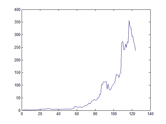
The problem is that historical data on both VXX and XIV are very limited (they go back only as far as late 2010). There is not much to do on Strategy 3), as VXV is a bottleneck. For Strategy 4)m though, I planned to retrospectively compute VXX and XIV prices pre-launch by using VIX future prices with their rebalancing rules. Fortunately the folk at The Intelligent Investor Blog has done exactly this, which saves me a lot of time and efforts. The following is the equity curve (start with $1; every time there is a signal, the liquidation amount is re-invested into the other ETN):
 As you can see, the performance is extremely appealing between 2004 (the earliest VIX future data one could find) up to late 2010. Since then, however, it has been a trip downhill all the way up until now. What was wrong? Is it indicating a regime change?
Strategy 3): Hold VXX when the VIX term structure is in backwardation; hold XIV when it is in contango; and
Strategy 4): Hold VXX when recent realized vol is greater than VIX; hold XIV when recent realized vol is less than VIX
where contango and backwardation are defined by the levels of VIX (30 days variance swap rate) versus VXV (3 month variance swap rate).
The problem is that historical data on both VXX and XIV are very limited (they go back only as far as late 2010). There is not much to do on Strategy 3), as VXV is a bottleneck. For Strategy 4)m though, I planned to retrospectively compute VXX and XIV prices pre-launch by using VIX future prices with their rebalancing rules. Fortunately the folk at The Intelligent Investor Blog has done exactly this, which saves me a lot of time and efforts. The following is the equity curve (start with $1; every time there is a signal, the liquidation amount is re-invested into the other ETN):
Thursday, February 28, 2013
Notes on Arbitrage
A lot of people and funds claim that they perform arbitrage in order to make a profit. Sometimes it is a little confusing because the term "arbitrage" is used by different individuals to mean quite different things (especially with terms such as stat arb). I think arbitrage can carry a few distinct meanings:
1. The real, good-old sure profit arbitrage
This refers to the option-pricing kind of arbitrage. The PnL is deterministic, since you are basically earning a sure profit by long-shorting the same security across different markets to exploit the price discrepancy. Examples would be a) trading the same contract listed on two exchanges when the prices diverge; and 2) synthesizing a contract (e.g. future) using something else (e.g. call and put).
2. Statistical arbitrage, looking at historical data
This refers to fitting a model to the historical performance. A classic example is pairs trading, in which the price of two assets are expected to return to the "normal" level when a deviation is observed. In a sense, this kind of arbitrage relies on the real world probability distribution as suggested by historical data.
3. Statistical arbitrage, looking at market data
This refers to fitting a model to the market prices. For example, one can try to see if the deep OTM options are over-priced or under-priced, by studying the Greeks. In a sense, this kind of arbitrage relies on the risk-neutral probability distribution as suggested by market data.
Monday, February 25, 2013
Book Review: Volatility Trading by Euan Sinclair
I first came across this book a few years back. I didn't put much time and thought on it back then but now that I revisit it, I find that it is actually quite a practical book for anyone who wants to investigate volatility trading.
The book covers a lot of ground, from basic vol trading principles to vol forecasting to hedging and bet sizing. Perhaps you will find that it tries too hard to be comprehensive, so feel free to skip some sections (such as Ch.8 Psychology).
Nonetheless, there are some good parts. In Ch.2 the author talks about different ways to measure volatility (different calculation methodologies, data with different frequencies etc.). These go beyond the most common definition of volatility, and are essential for creating useful and relevant estimators.
Of particular interest is the section on forecasting volatility. Here Sinclair explains the merits and shortcomings of GARCH type models from a practical point of view. The volatility cone is introduced, and although some might find it too heuristic and ad hoc, it does provide a relatively simple and systematic way to bring implied vol and realized vol into comparison.
The chapter on vol surface dynamics is quite weak, which is possibly a price to pay by not including too much theory. However the chapter on hedging is definitely worth a read, as it is not so much a crash course on Greeks calculation, but rather an in-depth investigation on why, what and when to hedge when trying to trade volatility.
http://www.amazon.com/Volatility-Trading-CD-ROM-Wiley/dp/0470181990
Wednesday, February 20, 2013
Those damn dice...
To recap, a dice rolling game contrasts with coin tossing in:
- Coin tossing follows a binomial distribution (which converges to Gaussian); die rolling follows a uniform distribution.
- Tossing m coins gives an expectation value of m/2; rolling an m-sided die gives an expectation value of (m+1)/2.
Since the probability distribution itself for dice game is simpler, the game you would encounter in an interview is usually more complex to compensate for it. Let's start with some easy ones.
DR01
Player A rolls one die for 4 times, aiming to get one 6; player B rolls two dice for 24 times, aiming to get (6,6). Who has a better chance of winning?
DR01 - Answer:
The probabilities are 1-(5/6)^4 vs. 1-(35/36)^24
DR02
When rolling 2 dice, what is P(both are 6 | at least one 6)?
DR02 - Answer:
Bayesian: (1 * 1/36) / (1 - 25/36) = 1/11
DR03
You have two dice, one is 10-sided and the other is 20-sided. What is P(points on 10-sided die > points on 20-sided die)?
DR03 - Answer:
(1 + ... + 9) / 200 = 9/40
See here for more interview questions/brainteasers
Tuesday, January 8, 2013
More Coin Problems
CT10
What is P(# of H out of 4 tosses >= # of H out of 5 tosses)?
CT10 - Answer:
1/2 (symmetry consideration)
CT11
Flip n unbiased coins. What is P(# of H = n/2)?
CT11 - Answer:
nC_(n/2)/2^n
CT12
Toss 4 coins and win the number of H. There is an option to re-toss. What is the value of the game?
CT12 - Answer:
([1 4 6 4 1] * [2 2 2 3 4]') / 16 = $2.375 (dynamic programming/backward induction)
CT13
What is the expected product of (# of H) * (# of T) when tossing 10 fair coins? (Hint: the answer is not 25)
CT13 - Answer:
22.5 (E[(# of H) * (10 - # of H)])
CT14
Keep flipping a fair coin. What is the probability that the sequence HHT appears before THH does?
CT14 - Answer:
1/4 (Once you have T, THH would always precede HHT; likewise, once you have HH, HHT would always precede THH)
CT15
Toss 4 coins and win the number of H. There is an option to re-toss one coin. What is the value of the game?
CT15 - Answer:
2 + 0.5 * 15/16 = $2.469 (dynamic programming/backward induction)
See here for more interview questions/brainteasers
Subscribe to:
Comments (Atom)