The Gamma-Theta story

• Gamma and theta are usually of opposite signs and of similar magnitude. This comes from the fact that they are on the same side of the pricing PDE, and other terms are usually smaller in magnitude.
• Suppose you are a market-maker selling a call option. The option value decreases with time, does that mean you can just sit there with your premium? No, you have to delta-hedge the short call position. And due to convexity of call option price with respect to asset price (it is actually CONCAVE when you are shorting), you lose a small bit whenever you adjust your delta-hedge discretely. At the end of the day if volatility stays constant at the original implied level, your premium should exactly cover this hedging cost.
• Similar story can be told from the other side (the option buyer), who would get her premium back when she delta-hedges. It is in these senses that theta is considered a 'cost' to purchase gamma, and vice versa depending on the position you hold.
• Of course, if realized volatility turns out to be varying, somebody would get hurt. Delta-hedging of a vanilla option is a way to capture volatility changes, but it is not effective due to path dependence.
  

Reference: Veronesi, Wilmott "Paul Wilmott on Quantitative Finance" Ch. 12

Variance Swap Revisited, Part II

1. Once again, a variance swap is not just the log contract. It's the log contract plus dynamically hedged $1 worth of stock.
2. Greeks of a variance swap (under B-S): Vega decreases linearly with time; Delta zero (but...); dollar Gamma constant.
3. Two disadvantages of straddle (even if delta-hedged), as compared to variance swap, are that 1) volatility exposure rapidly diminishes as soon as asset price moves away from strike; and 2) path dependence of P&L.
4. Due to these subtle differences between variance swap and delta-hedged straddle, the combination of the two is a neat way to trade the variance convexity. However the moving-underlying problem is still present and the delta-hedged straddle leg of this trade has to be periodically re-struck.
5. Taking a step back, the reason why volatility capturing using vanilla option (or a porfolio of them) depends on path is that the Gamma of the option/options changes as underlying moves.
6. Interest rate term structure has a short end (short rate) that is quite stable; on the other hand the short end of the variance term structure can move substantially and abruptly.

Reference: JP Morgan Variance Swap
Further readings: Correlation trading, volatility skew trading using Gamma swap

Variance Swap Revisited, Part I

1. Why is it that Vega Notional = 2K *Variance Notional? Because when calculating P&L, (sigma^2 - K^2)/2K is roughly "d sigma". This approximation, of course, is linear and is good only when close to strike, which brings us to...
2. CONVEXITY. Variance swap payoff is convex with respect to volatility. The further away realized variance is from the strike, the more pronounced the effect of convexity is. This means that 1) the fair strike for a variance swap is always greater than the fair strike of a comparable volatility swap because of the benefit of convexity; and 2) Variance swap price increases with vol-of-vol, but volatility swap price does not.
3. The forward arithmetic of IR is mutiplicative; the forward arithmetic of variance is additive.
4. For capped variance swaps, unwinding by entering into an opposite trade is complicated by the fact that the cap itself would move when one tries to lock in the P&L after some time, causing the offsetting trade to have a different cap level than the original trade.
5. Derman's approximation assumes that implied volatility curve is linear. This approximation is good when vol-of-vol effect is low, e.g. for shorter-term index variance swap (instead of single stock variance swap)
6. Volatility risk premium: the price of variance swap is 'too high' as compared to both historical realized volatility or implied vanilla option volatility. In other words longing variance is in high demand. Not to be confused with the vol-of-vol effect.
7. Variance swap can be replicated by OTM call and put options, hence the fair strike is a weighted average of implied variances across the entire volatility smile, which, given a volatility smile (going up both ways), is greater than sigma_ATM.

Reference: JP Morgan Variance Swaps

Vanna-Volga Approximation

Vanna-Volga approximation is the quick-n-dirty way traders use to tweak B-S price so that smile/skew effects are taken into account. It is used to price exotic products. It consists of 3 components: X_BS, RR (risk reversal) correction and BF (butterfly) correction. Incidentally, unlike in equity market where the smile is simply quoted from the market, the FX market convention is much more convoluted, with only ATM, RR and strangle volatilities directly quotable (note also the RR and strangle and BF volatilites are not really volatility in the strict sense; they are merely traded entities).

• X_BS is the B-S exotic price
• RR stands for risk-reversal. An RR strategy consists of long OTM call and short OTM put.
• BF stands for butterfly. A BF strategy consists of long strangle and short straddle.

Intuitively, RR and BF have opposite parity about the strike (RR increases monotonically, BF increases either way). Hence they together can produce corrections that fit market prices. In fact, RR strategy has large (small) vanna (volga) exposure, while BF strategy has large (small) volga (vanna) exposure (this can be seen by considering the B-S Vega expression, Vega ~ S phi(d_1)). The Vanna-Volga method ignores the cost of hedging Vega.

*Volga = (d/d sigma) Vega, Vanna = (d/dS) Vega

Reference:
Bossens 2010 - Vanna-Volga method
Reiswich 2010 - Constructing a (quadratic) smile using the market quoted volatilities

Negative duration of FRN

Floating Rate Note (FRN) usually has duration very close to zero. An FRN is reset to par on every reset date when the floating coupon is paid out. However it could have negative duration when it is traded at substantial discounts. Since, as we have already mentioned, the coupon of an FRN is floating, the discount is most probably due to credit instead of interest rate. Suppose then that an FRN is traded at a discount because of credit concern. Then we can write

FRN = FRN' + X

where FRN' is a note at a discount, FRN is an otherwise identical par note and X is some instrument that can be constructed so that the above expression holds. The point is that X has positive duration (as can be shown easily if we assume that the cash flow of FRN' is that of FRN with an extra spread S). Since the duration of FRN is close to zero, and the duration of X is positive, we must have that the duration of FRN' is negative.

(Possible) Quant Interview Questions

1. Maths
What is i^i? Give your answer to 2 decimal places for both the real and the imaginary parts.

2. Black-Scholes
Assume Black-Scholes and no dividend. P and C are, respectively, European vanilla put and call that are otherwise identical. What is the strike price that would make
i) their price; and
ii) their delta
the same?

3. Fixed income
The current yield curve is upward sloping. You speculate that it will get steeper and want to take advantage of it by long-shorting zero coupon bonds with different maturities (5 yrs and 10 yrs).
i) What is the duration-neutral strategy?
ii) What is the impact to your duration-neutral portfolio if there is a small parallel shift in the yield curve? A large (>>1bps) upward shift? A large (>>1bp) downward shift?

See here for more interview questions/brainteasers

Analogies have their limitations

CDS and IR swap are very similar in many aspects. However one must also be aware of where the analogy ends. As an example, one can lock in the profit of a pay-fixed swap (when swap rate goes up) by entering into a receive-fixed swap, IF THE SWAPS ARE RISK-FREE. Alternatively she could unwind the position (selling the swap) and collect the present value of the cash flow.

For CDS things are more complicated. Unwinding the position would still let the investor cash-out immediately. Entering into an opposite swap, however, does not guarantee the cash flow anymore because there is the possibility of default, which would terminate the cash flows from both positions (the original protection buyer and the opposite seller).

Short note on ways to avoid negative short rate

- BK, BLT or other exponential-Gaussian models
- Imposing absorbing or reflecting BC (Goldstein and Keirstead)
- Kim and Singleton reviewed a few possibilities:

• Affine models like CIR, under which zero is not accessible
• Quadratic Gaussian models
• Black's shadow rate (i.e. treating bond yield as a call option to a latent process that CAN go negative)

MC Simulation for Hull-White Model

Recipe 1
Fit kappa and sigma by calibrating to swaptions/caps (swaption and cap prices can be expressed as Hull-White bond options, which in turn can be expressed as function of H-W bond price). Then calculate theta(t) by taking partial derivative of instantaneous forward rate f(0,t). Then do Euler MC simulation:

$r(t)=r(s)+(\theta (t) - \kappa r)dt + \sigma dW$

Recipe 2
This alternative method doesn't require taking partial on f(0,t). After fitting kappa and sigma,
then do the following MC simulation (it is by integrating the SDE):

$r(t)=r(s)e^{-\kappa (t-s)} + \alpha(t) - \alpha(s)e^{-\kappa(t-s)}+B$

where B is a Gaussian distributed white noise with variance

 $ \frac {\sigma^2}{2 \kappa} [1-e^{-2 \kappa (t-s)}]$

and

$\alpha(t) = f(0,t) + \frac {\sigma^2}{2\kappa^2}(1-e^{-\kappa t})^2$

Bottom line is, theta-fitting is about calibrating to the spot curve. But Recipe 2 does just that without invoking theta, because the instantaneous forward rate contains the same information.

Ref: Brigo pp.73

Also:
One can simulate the stochastic short rate process under the T-forward measure instead of the risk-neutral measure. The drift of the SDE will be different from that above, and would depend on T.

Advantage:
Since under the T-forward measure we discount the payoff with zero coupon bond, and the zero coupon bond price is completely determined by the short rate at a certain moment, we don't have to simulate too many points on a path, but we do need to do that for risk-neutral measure pricing in order to approximate the money-market account well.

Disadvantage:
P(t,T) bond is the natural numeraire to use for discounting, but what if we are pricing an instrument with multiple cash flows?

Short note on Vasicek CDO pricing model

- It is a PRICING model, not a credit default rate model (i.e. neither structural nor reduced-form, it takes prob. of default as input)
- It assumes (in its most simple form) large, homogeneous pool
- It assumes Gaussian copula (can be relaxed)
- Just like B-S option pricing has implied volatility, Vasicek CDO pricing has implied correlation
- In its simplest form, the correlation matrix is assumed to be time-independent and all pairwise correlations are identical
- Industry people use Vasicek implied correlation as a convenient way to quote tranche price (cf. Black volatilities for cap/floor/swaption)
- Not surprisingly, the implied correlation is not constant across tranches - correlation smile
- Base correlation is smoother than compound correlation

Ref: This article by Elizalde

Shadow Rate

The original paper by Gorovoi and Linetsky, and a summary of it, is a pretty neat idea to resolve the shortcoming of Gaussian short rate models: that the interest rate can go below zero (but should we be concerned about negative rate, now that CHF Libor has seen negative values?).

The 'shadow rate,' which is a latent unobservable process, is still assumed to be Gaussian. The true short rate process is floored at zero of the latent process. Intuitively, people can always choose to hold cash when rate is below zero so the effective rate should never drop to negative.

They also use an eigenfunction expansion method to construct the solution to the PDE (derivative price).

(Original?) Brain teaser

There are 2 apartments, A and B. Apartment A has 10 tenants and 2 washing machines; apartment B has 20 tenants and 4 washing machines. If your objective is to minimize the probability that all machines are occupied when you want to do laundry, which one is better, A or B, or does it not matter? Assume that ‘Tenant i does laundry at time t’ follows mutually independent Poisson processes. Assume also that each and every laundry takes the same finite amount of time T.

Physical vs. Risk-neutral Measures in BSM Credit Model

Unlike in equity or fixed income derivative pricing, the concepts of hedging and portfolio replication are usually bypassed in credit modeling, especially when structural models are considered (although Vaillant 2001 discusses replicating credit derivatives using risky bonds, which mirrors replicating interest rate derivatives using risk-free bonds). To facilitate discussion we consider the BSM asset default boundary model. Usually we would ignore the nuances of probability measures and presume physical measure when writing down the asset dynamics. This produces the Distance to Default (DD) under the physical measure, which allows us to compute the Probability of Default (PD) under the physical measure. This is all very well, but when we want to calculate bond (or other security) prices using PD, we have to first convert the PD under P-measure into the PD under Q-measure. Bohn's Active Credit Portfolio Management pp. 177 explains this.

Ginnie Mae, Fannie Mae and Freddie Mac

Ginnie Mae
- does NOT hold any bond
- does NOT originate MBS
- does guarantee MBS issued by banks with the right ingredients
- is backed by 'full faith of the government'

Fannie Mae and Freddie Mac
- does hold some bonds
- does originate MBS
- does guarantee MBS issued by banks with the right ingredients*
- (formally speaking) is NOT backed by 'full faith of the government

Note*:
1. Fannie Mae and Freddie Mac guarantee bonds, whether they are their own originations or not
2. "Right ingredients" here are different from those in Ginnie Mae guaranteed MBS

The volatility of corp bond yield

Q: How does the volatility of the yield of corporate bond compare to that of treasuries?

A: The question can be translated into "is the correlation between corporate yield spread and the underlying index yield (treasury yield) positive or negative?" Empirical study shows that they are negatively correlated. What is the economic story? When the underlying riskless treasury yield is high, the general economy is usually doing well (i.e. what is the objective of the Fed?) and so the corporates are in good shape to service their debts. Default is therefore less likely.

Since the correlation is negative, the answer to the original question is that the yield of corporate bond actually tends to be lower than that of treasury securities. This is a little anti-intuitive, as we expect the corporate bond to be riskier and hence has more volatile price.

Quant Interview Questions (Interest Rate Strat.)

1) What is the limit of F(n) when n is large, where F(n) is the n-th term in the Fibonacci series?

Ans:
The ratio between consecutive terms, x, approaches the golden ratio phi. Proof: we posit that
F(n) = x^n * F(0) = x^(n-1) * F(0) + x^(n-2) * F(0)
x^n = x^(n-1) + x^(n-2)
x = 0.5 * (1 +- sqrt(5))
The two values are phi and 1/phi, respective.

2) Write functions to compute F(n) and comment on the order of the algorithm.

Ans:
Recursive approach -
int Fib(int n){
if (n = 0) {Fib = 0}
else if (n = 1) {Fib = 1}
else {
Fib = Fib(n-1) + Fib(n-2)
}
return Fib;
}
Order ~ O(phi^n)
Note: alternatively we can store the intermediate values in a cache to reduce redundancy (for example to find F(4) we have to calculate F(2) = F(3-1) and F(2) = F(4-2) twice, which is a waste of time).

Bottom-up approach -
int Fib(int n){
temp1 = 0;
temp2 = 1;
if (n = 0) {Fib = 0}
if (n = 1) {Fib = 1}
for (int i = 0; i <= n; i++){
run_sum = temp1 + temp2;
temp1 = temp2;
temp2 = run_sum;
}
return run_sum;
}
Order ~ O(n)

See here for more interview questions/brainteasers

Quant Interview Questions (Equity Exotic Derivatives)

1) What is the Taylor expansion of exp(-1/x^2)?

Ans:
This function cannot be expanded at x = 0 because there is a singularity: the function is NOT analytic at x = 0.
http://en.wikipedia.org/wiki/Taylor_series#Analytic_functions

2) Suppose we have the prices of options with various strikes. How can we price an option with arbitrary payoff?

Ans:
Solve the Fokker-Planck Equation to obtain the risk-neutral probability density p(S). Then the price of an option with arbitrary payoff can be calculated as
exp(-r (T-t)) \int Payoff(S) p(S) dS
Note: In case of vanilla European call, p(S) can be found by the second partial derivative of the call price w.r.t. strike K

3) Suppose we have a volatility smile (same expiry, different strikes). What no-arbitrage condition can be imposed on the option implied volatilities (i.e. prices)?

Ans:
Recall the bull spread relation and the butterfly spread relation. In the continuous limit, they read
0 < -dC/dK < 1 [Note the negative sign]
d^2C/dK^2 > 0

4) Given two stock price time series of two stocks. After computing the correlation using the naive approach (rolling covariance divided by rolling standard deviations), the correlation matrix is NOT PSD. How can this be fixed?

Ans:
??

See here for more interview questions/brainteasers

Barrier and Asian Options

In hedging barrier and Asian options, we do not need an extra asset in addition to the underlying stock. That is to say, although the payoff and value of the barrier (Asian) option does depend on the running extremum (average) process, such a process does not introduce an extra source of uncertainty (however they do introduce an extra dimension in numerical pricing).

- For barrier option, the running extremum can be handled using reflection principle.

- For Asian option, the running average can be handled by having an auxiliary process. Once again, no additional source of uncertainty is introduced by doing this.

See Shreve.

C++ Advanced Concepts

1) Initialization List
http://www.learncpp.com/cpp-tutorial/101-constructor-initialization-lists/
Also, http://www.cprogramming.com/tutorial/initialization-lists-c++.html:
"Before the body of the constructor is run, all of the constructors for its parent class and then for its fields are invoked. By default, the no-argument constructors are invoked. Initialization lists allow you to choose which constructor is called and what arguments that constructor receives.

If you have a reference or a const field, or if one of the classes used does not have a default constructor, you must use an initialization list."

2) Overloading Function and Copy Constructor
http://www.learncpp.com/cpp-tutorial/911-the-copy-constructor-and-overloading-the-assignment-operator/

3) Virtual Constructor Function
See Eckel "Thinking in C++":
"If you want to be able to call a virtual function inside the constructor and have it do the right thing, you must use a technique to simulate a virtual constructor. This is a conundrum. Remember, the idea of a virtual function is that you send a message to an object and let the object figure out the right thing to do. But a constructor builds an object. So a virtual constructor would be like saying, “I don’t know exactly what kind of object you are, but build the right type anyway.” In an ordinary constructor, the compiler must know which VTABLE address to bind to the VPTR, and even if it existed, a virtual constructor couldn’t do this because it doesn’t know all the type information at compile time. It makes sense that a constructor can’t be virtual because it is the one function that absolutely must know everything about the type of the object.

And yet there are times when you want something approximating the behavior of a virtual constructor..."

4) Virtual Destructor
Why we need virtual destructor is exactly because of polymorphism. Consider if we have BaseClass and ChildClass. If we do this:

BaseClass *p = new ChildClass;
delete p;

then we fail to delete the ChildClass object! Although the pointer of the BaseClass can point to an object of the ChildClass, the command delete could only get rid of a BaseClass object - unless it has a virtual destructor!

http://blogs.msdn.com/b/oldnewthing/archive/2004/05/07/127826.aspx

5) Avoiding changing value when passing by reference
Use the technique of passing by const reference (http://www.learncpp.com/cpp-tutorial/73-passing-arguments-by-reference):
"One of the major disadvantages of pass by value is that all arguments passed by value are copied to the parameters. When the arguments are large structs or classes, this can take a lot of time. References provide a way to avoid this penalty. When an argument is passed by reference, a reference is created to the actual argument (which takes minimal time) and no copying of values takes place. This allows us to pass large structs and classes with a minimum performance penalty.

However, this also opens us up to potential trouble. References allow the function to change the value of the argument, which in many cases is undesirable. If we know that a function should not change the value of an argument, but don’t want to pass by value, the best solution is to pass by const reference."

cf. http://iagtm.blogspot.com/2010/02/c-function-passing-by.html

Quant Interview Questions (Model Validation 2)

1) Consider the SDE dr = a r dt + b dW. What is the solution for r?

Ans:
This is a special case of O-U process. Try taking derivative of $ f \equiv r_t e^{-at} $

2) Toss a fair coin for 100 times. What is (approximately) the probability Pr(# of H >= 60)?

Ans:
Consider the binomial distribution
n C k*p^k*(1-p)^(n-k)
The mean of the distribution is n*p and the variance is n*p*(1-p). When n is large, the binomial distribution converges to normal distribution with mean = n*p and variance = n*p*(1-p). Hence the standard deviation in this case is 5, and H >= 60 would be two standard deviation away from the mean. The answer is therefore (1 - 95.4%)/2 = 2.3%.

3) What is copula and how can it be used for modeling correlated processes?

Ans:
Let F_X and G_Y be the cdf of random variables X and Y, and they are the marginal distribution of the bivariate distribution H_XY. Using the fact that U = F_X(X) and V = G_Y(Y) both have uniform distribution from 0 to 1 (because F_X(X) is the percentile function). Sklar's Theorem states that there exists a copula function C such that
H_XY = C(F_X, G_Y)
In other words, we can construct the joint distribution using the marginal distributions.

Reference: http://en.wikipedia.org/wiki/Copula_%28statistics%29

4) Why is holding the equity piece of a CDO longing default correlation?

Ans:
Holding the senior tranche is a short position in correlation - that is easy to understand, because the probability of loss for the senior tranche is low as long as not too many assets in the pool default together in a bad credit environment. However, for the equity piece it seems that it will not actively benefit from high correlation. The way to think of it is to consider when credit environment is good, a high correlation ensures that no asset in the pool goes default.

5) Suppose x is a continuous observable variable, Y* is a binary observable variable, and Y is a latent variable. The following relations hold:
Y = b x + e, e ~ N(0,1)
Y* = 1 (if Y >= 0) or 0 (if Y < 0)
Suppose we have a set of data (x, Y*). How can be calibrate the model (i.e. fit b)?

Ans:
This problem can be solved by MLE. Since e ~ N(0,1), we have Y ~ N(b x, 1). The probability of Y* = 1 (or equivalently Y >= 0) is just the cumulative normal probability density. For each of the data point (x_i, Y*_i) we have such an F(Y). Thus the likelihood function is
Product(F_i(Y))
and we fit b by maximizing this function.

6) A, B and C are playing a game with gemstones. Each of them starts with 5 stones with different colors (blue, red, green, yellow, white). There are 3 rounds in the game. In the first round, A pick one stone randomly from B and one from C; in the second round B pick one stone randomly from C and one from A; in the third round C pick one stone randomly from A and one from B. What is the probability that at the end of the game each person would have 5 stones with different colors?

Ans:
0.015873 (MC verification)
Edit: Thanks to M Millar, the right answer should be 0.0413. The tree looks like
                                                                                                  -- C gets the right stones (1/9)
                                            -- B takes original from A (3/7) --
                                           |                                                      -- C fails (dead)
   -- A draws same color (1/5) --
  |                                         -- B fails to take original from A (dead)
--
  |                                        -- B takes original from A (2/7) -- C gets the right stones (1/9)
  |                                       |
  |                                       |                                                         -- B takes the right color from C (1/4) -- C gets the right stones (1/9)
   -- A draws diff colors (4/5)  ---- B takes the other duplicated color from A (2/7) --
                                          |                                                         -- B takes the wrong color from C (dead)
                                           -- B removes one of the three lone colors (dead)


See here for more interview questions/brainteasers

Quant Interview Questions (Interest Rate Strat.)

1)
Suppose you have a fair coin. How do you create an event A such that Pr(A) = 1/3?

Ans:
Toss the coin twice to produce the following space: {HH, HT, TH, TT}. Discard one of the element in the set. Each of the remaining outcome represents an event A.

Note: This recipe can be extended to producing an event with probability m/n, m and n being integers.

2)
Suppose you have a fair coin. How do you create an event A such that Pr(A) = r, r being an irrational number between 0 and 1?

Ans:
Translate r into a binary string. For example, 0.27314... would be {10}{0111}{011}{01}{100}... We start tossing the coin until we can tell if the string formed by coin tossing is greater/less than r in binary, with H = 1 and T = 0. For example, the first step is to toss twice. If we have {TH} = {01}, then the string formed by coin tossing must be less than r in binary. We terminate and conclude that the event belongs to A; If we have {HH} = {11}, then the string formed by coin tossing must be greater than r in binary. We terminate and conclude that the event does not belong to A. If the two tosses produce {HT} = {10} then we cannot conclude, and have to move on to the next digit {111}, and so on. (MC verification)

Note: We have to append a zero in front of {111}, {11} and {1} because otherwise we cannot create a greater binary, i.e. 111 is the greatest 3-digit binary number.

See here for more interview questions/brainteasers

Quant Interview Questions (Model Validation)

1) Suppose Prob(Tail) = p. What is the probability distribution of N, where N is the event:
The first Head shows up at the N-th toss.

Ans:
The (discrete) probability density is simply
Pr(event) = p^(N-1) (1-p)

What is the expectation value of N?

Ans:
E[N] = Sum_(i=1)^(inf) i*p^(i-1) (1-p)
How to do this sum? Trick:
i*p^(i-1) = (d/dp)p^i
Using this and exchanging the order of summation and differentiation, we get
E[N] = 1/(1-p)

2) Suppose X and Y are two random variables with the same cdf, X, Y > 0 and E[X/Y] = 1. Show that E[X] = E[Y].

Ans:
Cauchy-Schwarz inequality, but how?

See here for more interview questions/brainteasers

About Stochastic and Not-So-Stochastic Integrals

Here we consider 3 kinds of integrals. Suppose W is a Brownian motion, f is a stochastic function and g is a deterministic function.

1. $ \int_t^T W_s ds $
This entity turns out to be a normally distributed random variable, distributed as N(0, $ T^3 /3 $). [Missing: proof , can be found in Crack's HOTS pp. 154]

2. $ \int_t^T g dW_s $
This is not only a martingale, but also a normally distributed random variable N(0,$ \int_t^T g^2 ds $).

3. $ \int_t^T f dW_s $
This is a martingale, but the distribution is not (necessarily) normal.

One implication of 2. versus 3. is this.

Ito Calculus Revisited

Most General Case
In d-dimensions, Ito's Lemma reads
Note that, unlike in the specific case below, the dynamics of the process X is NOT specified.

Specific Case
In one-dimension and assuming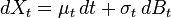Ito's Lemma reads
Notes: Partial f partial t comes from the fact the f is defined as f(t,X). cf. the general case above, where f=f(X). This so-called one-dimensional case is in fact 2-dimensional, with one of the dimension being deterministic (time).

Ito's Product Rule
Suppose X and Y are processes driven by the same Brownian motion. Then
where d[X,Y]=dXdY.
Note: This can be easily derived by considering a 2-dimensional Ito's Lemma, where f(X,Y)=XY.

Source of formulae images:
http://en.wikipedia.org/wiki/It%C5%8D_calculus
http://en.wikipedia.org/wiki/It%C5%8D%27s_lemma

Structural vs Reduced-Form Models (Credit)

Structural Models:
Considers default as being driven by the firm's assets.
Example: Merton
Note: Structural Models produce poor bond prices, but OK to use them to calculate PD.

Reduced-Form Models:
Proposes a relationship between bond price/yield and default risk. Default risk proxied by hazard rate. Then use market price to back out the hazard rate (hazard rate term structure fitting).
Example: Duffie and Singleton (1999)

Structural vs Reduced-Form Models (ABS)

Structural Models:
Treats prepayment as a (American) call option of the mortgage. Tries to solve for the optimal exercise strategy. Focuses on why loans terminate. Needs full information set for calibration (i.e., not just market prices). Computationally too expensive to be practical. Some primitive Structural Models do not allow for mortgages to exceed par.
Example: Dunn and McConnell (1981)

Reduced-Form Models:
Focuses on how (or, when) loans terminate. Needs only partial information set for calibration. Poor out-of-sample performance. Often are hazard models.
Example: Schwartz and Torous (1989)

Quant Interview Question

There are 2 pills A from bottle A and 2 pills B from bottle B. You have to take 1 pill A and 1 pill B every day, for two days, to survive. After taking 1 pill A from bottle A, you accidentally retrieved 2 pills B from bottle B. Now you have 3 indistinguishable pills in your hand (you do know that 1 out of the 3 is A and the rest are B). What's your survival strategy?

Ans:
Cut all 3 indistinguishable pills in halves (6 half-pills in total) and separate them into two piles. Make sure that each pile only contains a half from each individual pill. Now, each pile would necessarily contain 0.5 pill A and 1 pill B. Take the remaining pill A (still in bottle A) and split that in halves. We have created two "daily-doses" (the two piles) of the right composition for survival, although we still do not know which pill is which type.

Remark:
This can be trivially extended to n pills, n>2.

See here for more interview questions/brainteasers

Instantaneous vs. Terminal volatility/correlation

Instantaneous vol. and correlation refer to the sigma and rho within the SDE's.

Terminal vol. and correlation require integrations. For an explanation on how instantaneous and terminal correlation differ, see Brigo pp.234-237.

Question to think about: are variance swap and correlation swap trading on instantaneous or terminal vol./correlation?

Trading Interview Questions

Brainteaser 1
There are N dice, each having x faces. What is the number of combination that give at least one 1 or x?
Ans: (x - 2)^N

Brainteaser 2
What is the longest diagonal within a k-dimensional hypercube?
Ans: sqrt(k)

Finance 1
You purchase a 5yr pure discount bond at 5% yield. One month later you sell it at 4% yield. What is the IRR of this investment?
Ans: ~60%

Finance 2
You enter into a pair trade consisting of CDS_A of 5yr tenor and 100bps, and CDS_B of 5yr tenor and 300bps. Suppose the spread narrows down to 100bps (from 200 bps) after 1 year and you are to unwind it. Describe the strategy and estimate the profit of this trade.
Ans: Sell protection with CDS_B and buy protection with CDS_A. Profit = 600bps (why?)

Finance 3
Part I
You, an American investor, are holding a 10yr convertible bond that is convertible over the first 5 years. Explain what risks you are exposed to and how they can be hedged away.
Ans:
a) Price risk (wrt the underlying equity). Can be hedged by shorting vanilla call.
b) IR risk. Can be hedged by shorting one (or more) zero coupon bonds, or entering into a fixed EUR for floating EUR swap.
c) FX risk. Can be hedged by entering into a floating EUR for floating USD swap.
NOTE: or we can enter into a fixed EUR for floating USD swap to hedge both IR and FX risks.
d) Credit risk. Can be hedged using CDS.
Part II
Suppose this is the only bond issued by the company. How do you calculate/estimate the price of a non-convertible 5yr bond issued by the same company?
Ans:
1. Strip away the embedded option to find the price of non-convertible 10yr
2. Find the spread of non-convertible 10yr over treasury curve/LIBOR swap curve
3. Here we have to make some sort of assumption regarding the term structure of the spread: constant, or usually slowing increasing
4. Using the spread term structure, find the spread of non-convertible 5yr over treasury curve/LIBOR swap curve
5. Using the spread of non-convertible 5yr over treasury curve/LIBOR swap curve, find the yield and hence the bond price

See here for more interview questions/brainteasers

LMM Calibration & Parameterization

Refer to Brigo Ch.6.

The 'calibration' of LMM to market data is trivial - since LMM is designed so as to be consistent with Black volatilities, the 'calibration' amounts to simply bootstrapping the caplet vol. from the cap vol.

However, we don't just want to use LMM to price caps/floors. We want to price other more exotic products. Hence we also have to specify the instantaneous volatilities (the diffusion coefficient sigma in the SDE) and the instantaneous correlations (the rho among the Brownian motions). Remember, if the payoff of an instrument depends on more than one LIBOR forward rates, then it depends on the terminal correlation, which in turn depends on both instantaneous volatility AND instantaneous correlation(Brigo pp.234). Note that we are assuming the scalar LIBOR specification (see here).

# LMM requires that sigma be deterministic. Hence parameterizing sigma amounts to choosing a deterministic function (of time) for the volatility term structure. Parameterizing sigma has nothing to do with fitting to market data.

# Meanwhile, correlation is a constant (matrix). By parameterizing the rho matrix we reduce the rank (i.e. degree of freedom) of the matrix. Parameterizing rho has nothing to do with fitting to market data.

Convexity, Time and Quanto Adjustments

Under the simplest B-S setting, the price of a forward contract does not depend on the volatility (cf. the price of a vanilla call). This makes sense because while the option payoff is asymmetric, hence would benefit from higher volatility, the forward payoff is symmetric (you lose money when the underlying price goes under water) and hence would neither benefit from nor be harmed by higher vol. However, in some cases the volatility comes into play even when the contract payoff is symmetric, and here we consider a few examples. The common theme of them is that we are trying to price an instrument under the "wrong" numeraire, which introduces an extra drift that does depend on the volatility.

Convexity/Time Adjustment
When the payoff is a linear function of the spot rate. The "wrong" numeraire is the zero coupon bond that does not expire on the right date (i.e. in-arrear swap or in-arrear cap/floor).

Quanto Adjustment
When the payoff is a linear function of the asset denominated in a foreign currency. The "wrong" numeraire is the domestic money-market account.

Reference:
Hull - Options, Futures and Other Derivatives [Chapter 29]
Veronesi - Fixed Income Securities [Section 21.7]
Brigo - Interest Rate Models [Chapter 13]

Polymorphism and Virtual Function in C++

Virtual function syntax:
virtual void func(int i){};

Pure virtual function syntax:
virtual void func(int i) = 0;

If a class contains at least one pure virtual member, it is an abstract class - we cannot instantiate an object of an abstract class. However, we can create a pointer that points to such a class. Suppose

class myAbsClass{
virtual void func(int i) = 0;
}

class myChildClass: public myAbsClass{
void func(int i) {return 1};
}

Then we can do
myAbsClass* pointer1;
pointer1 = new myChildClass;

Polymorphism makes coding more flexible and efficient. For example, suppose there are more than one (non-abstract) child classes, and each of them has different implementations of the virtual function in the parent class. If we want to write a function that requires the returned value of such functions, we do not have to write it multiple times, but only need to write it so that it takes the abstract pointer as an input.

Fixed Income Mathmetics

LIBOR rate and Bond price
L(t,S,T) = -(p(t,T) - p(t,S))/((T-S) p(t,T))
* LIBOR is just discretely compounded forward rate

Continuously compounded forward rate and Bond price
R(t,S,T) = -(log(p(t,T)) - log(p(t,S)))/(T-S)


Instantaneous forward rate and Bond price
f(t,T) = -d(log(p(t,T)))/dT

Instantaneous short rate
r(t) = f(t,t)

Bond price and Instantaneous forward rate
p(t,T) = exp[-\int^T_t f(t,s) ds]
Note: this is just the inversion of the f vs. p formula above

Bond price and Instantaneous short rate
p(t,T) = E^Q[exp[-\int^T_t r(s) ds]]
Note: this comes from valuing a 1 dollar payoff under the Q-measure

Different Rates

- Federal Funds Rate
Bank lending Fed funds to other banks

- Prime Rate
Bank lending money to its customers

- Repo/Discount Rate
Fed lending its own money to banks
See: Discount Window

- LIBOR (London Interbank Offered Rate)
Bank lending money to other banks

- OIS (Overnight Indexed Swap)
Banks paying/receiving floating/fixed with other banks
Note: The swap rate is usually in between LIBOR and the Fed funds rate
See: OIS

- Eurodollar
Banks lending USD outside US

What does the LIBOR-OIS spread tell us?
Both LIBOR and OIS are between two risky counterparties, but OIS is less risky (because of swap payment and nominal amount netting). Hence the LIBOR-OIS spread is a measure of banks' credit risks.

Thoughts/Summary on LMM

As compared to short rate models:

In short rate models, we are trying to infer derivative prices by considering the dynamics of the short rate (bottom-up). For LMM the approach is more like top-down: since the market has always been using the Black76' convention to quote cap and floor prices (volatilities), why not play along and jump on the bandwagon, pretend that the forward rate really behaves like a tradable asset and follows a GBM, and develop a set of forward rate dynamics that rules out arbitrage?

Notes:

1. The fact that forward rate F(t,T_1,T_2) is a martingale under the T_2 forward measure follows from the definition of forward rate F(t,T_1,T_2) = (p_1-p_2)/(tau p_2); while the fact that we demand F(t,T_1,T_2) follows a GBM (instead of, say, arithmetic BM) is to make it coincide with market quoting convention (Black76'). F(t,T_1,T_2) being martingale does not necessarily require F(t,T_1,T_2) follows GBM.
2. Bottom line: when using LMM we are not really thinking about forward rates evolving according to GBM; LMM is a way to be consistent with the market (in other words, preclude arbitrage given the Black pricing convention).

LIBOR Market Model: notation and specification

Reference: Bjork Ch.27

Two ways of specifying a LMM:
1) dL_i = L_i sigma_i dW^i
where
L_i = the i-th forward rate
sigma_i = a VECTOR of deterministic volatility
dW^i = k-dimensional Wiener process

Here dW^i is under the i-th forward measure. However, all forward rates are driven by the SAME Wiener process, albeit martingale is attained only when the rate is expressed under its own forward measure.

2) dL_i = L_i sigma_i dW_i
where
L_i = the i-th forward rate
sigma_i = a SCALAR of deterministic volatility
dW_i = 1-dimensional Wiener process


Note:
In 2), a correlation structure dW_i dW_j = rho_{i,j} is also required. Here, each forward rate is driven by its own Wiener process dW_i.

Local Vol. Pricing

How:

Find a function sigma(S,t) such that the existing market vol. surface is reproduced (fitting to option prices). At each point on the (S,t) plane, the B-S pricing equation is valid.

The subtlety is that although we set out to find sigma(S,t), the observable quantity is sigma(K,T-t).

Pro:

We don't have to introduce new stochastic processes. Market is still complete, and hence preference-free pricing still works (i.e. no need to guesstimate market price of risk of any kind).

Reference:
Derman's GS Research paper

Interview Question

Suppose you have an unfair coin, with probability of a head p ~ uniform(0,1). What is the probability of getting 2 (or n) heads?

Hints: For 2 heads the answer is not 1/4.

Ans: The answer is 1/3 for 2 heads and 1/(n+1) for n heads. Just integrate
\int_0^1 p^n U(0,1) dp = 1/(n+1)
The implication is that under uniform distribution, TH and HT are not distinguished.

See here for more interview questions/brainteasers

Durations

Duration: parallel yield curve shift
D = -(1/P)(dP/dr)

Modified duration:
MD = -(1/P)(dP/dy)

Macaulay duration: under the mindset of "duration<->time to maturity"
MacD = MD*(1+y/2)

Effective duration:
For securities with embedded options

Spot rate duration:
Spot rate is changes (not shift of the entire yield curve). Usually found numerically.

Factor duration:
Price change with respect to some factors other than rate

Also, since D = (-1/P) (dP/dy) and convexity C =  (1/P) (d^2P/dy^2), it can be shown that

dD/dy = D^2 - C