Recently re-read two very good papers (see the bottom), and it's interesting to find that they have related themes.
Synopsis for Jarrow: A model can either be theoretical or statistical (think regression). A theoretical model can be rejected (or not) by inspecting the assumptions and implications (note, though, that a rejected model can still be used). If a theoretical model is rejected, then calibration to market data would effectively turn it into an ad hoc statistical model.
For the sake of discussion consider B-S. It sets out to be a theoretical model, but volatility smile renders it rejected. By calibrating it to the volatility smile (local volatility), we are turning it into a statistical model. It can then be used to price other options (although, now being a statistical model, the econometric relationship would change over time and re-calibration is required). What we should not do is to use it for Delta/Gamma hedging, because it is exactly the failure of Delta hedging assumption that breaks its theoretical model status - there exist more than one sources of risk, which is why a single constant sigma does not suffice.
What is worse than using it for Delta hedging is to use it for Vega hedging, because under B-S the stock volatility is assumed to be a constant. Taking partial derivative with respect to sigma is mathematically sound, but it makes no sense other than spitting out an expression that lure you into believing its legitimacy. Which brings us to the uncertain parameters model Wilmott discussed. In his paper (and his book too) he explains why Vega is a terrible measure of volatility sensitivity when Gamma changes sign. Besides cliquet option, barrier option also falls into this category.
He proposes an uncertain parameter model that still uses Delta hedging argument. A non-linear PDE is produced. In a related chapter he discusses a similar technique for interest rate modeling, although in that case Delta hedging is dropped and the result of calibration is a yield envelop.
Jarrow 2011 - Risk Management Models: Construction, Testing, Usage
Wilmott - Cliquet Option Pricing
Also, PWOQF Ch. 52
Friday, February 10, 2012

Tuesday, February 7, 2012
Quick Notes on IR/Credit/Volatility Comparison
Modeling Approaches
Stochastic instantaneous spot
Short rate - Hazard rate - Stochastic volatility
Stochastic instantaneous forward
Instantaneous forward rate - ??? - xi in the Bergomi model
Market traded
LIBOR/Forward swap rate - Forward CDS rate - Forward variance swap rate
Others (Not exactly modeling)
Yield - ??? - Implied volatility
Question: where does local volatility fit in?
Stochastic instantaneous spot
Short rate - Hazard rate - Stochastic volatility
Stochastic instantaneous forward
Instantaneous forward rate - ??? - xi in the Bergomi model
Market traded
LIBOR/Forward swap rate - Forward CDS rate - Forward variance swap rate
Others (Not exactly modeling)
Yield - ??? - Implied volatility
Question: where does local volatility fit in?
Saturday, January 14, 2012
Stochastic Volatility One-Period Tree
We have three securities (money market account, stock, call option on the stock with K = 100). Today their prices are [100, 100, 8]. Suppose one period from now the stock can end up being either in the high-volatility (in which case S = 120 or 80) or low-volatility (in which case S = 110 or 90) regime.The MMA would still be 100. Now consider an exotic option X. The payoff of X is (30, 0, 0, 15) corresponding to (high vol stock up, high vol stock down, low vol stock up, low vol stock down). You can imagine it as a derivative that becomes a call when volatility is high and a put otherwise. What is today's value of X?
Ans: $12
Note: This problem is solvable because the matrix that represents basis securities payoffs has a left inverse. When would this be not true? -> When some basis security is the linear combination of others.
Ans: $12
Note: This problem is solvable because the matrix that represents basis securities payoffs has a left inverse. When would this be not true? -> When some basis security is the linear combination of others.
Thursday, January 12, 2012
Great link on swap spread
http://fermatslastspreadsheet.wordpress.com/2012/01/11/facts-intuition-and-rules-of-thumb-for-swap-spreads/
Not just introduces the concept but also discusses how to put it in credit/rates trading context.
Not just introduces the concept but also discusses how to put it in credit/rates trading context.
Tuesday, January 3, 2012
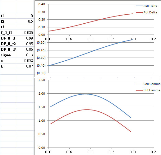
Short Rate Delta & Gamma (Hull-White One Factor)
Selection of European bond option greeks plots.
t2: option expiry
t3: underlying maturity
sigma: H-W volatility
a: H-W mean reversion
k: strike
x-axis: short rate




Pricing Callable Coupon Bond
Pricing a European callable zero-coupon bond is relatively straight forward. In fact, the callable zero-coupon bond can be decomposed into a non-callable zero-coupon bond and an European call option. Under many models (e.g. Hull-White), closed-form solution exists for European call option written on zero-coupon bond.
However, in reality, most callable corporate bonds bear coupons and the embedded options are American. In this case pricing would be much more complicated. First of all, since the embedded options are American, optimal exercise has to be considered. Secondly, the call on the principal plus the coupons cannot be seen as a basket of options because the option holder could only exercise the right to call everything, not an individual piece of cash flow.
There are at least 3 ways to tackle the pricing of callable coupon bonds:
However, in reality, most callable corporate bonds bear coupons and the embedded options are American. In this case pricing would be much more complicated. First of all, since the embedded options are American, optimal exercise has to be considered. Secondly, the call on the principal plus the coupons cannot be seen as a basket of options because the option holder could only exercise the right to call everything, not an individual piece of cash flow.
There are at least 3 ways to tackle the pricing of callable coupon bonds:
- Structural model - much like the structural credit models, we can postulate a model that describes how exercise strategy and hence option price are affected by the goal to minimize firm liabilities, by assuming a stochastic firm value process. Like other structural models, the drawback is that complete firm information is required.
- Reduced form model (American option) - this is similar to the pricing of callable zero-coupon bonds, namely by explicitly considering the embedded call. The drawbacks are that a) the bond can never exceed par (the same problem arises in MBS reduced form pricing), and b) numerical method is necessary.
- Reduced form model ("call intensity") - Jarrow et al proposes a method that treats the call feature as a hazard besides credit default risk. The approach is very similar to the reduced form model of Duffie and Singleton 1999. If the call intensity process is affine, closed-form solution exists.
Saturday, November 26, 2011
The Gamma-Theta story
- Gamma and theta are usually of opposite signs and of similar magnitude. This comes from the fact that they are on the same side of the pricing PDE, and other terms are usually smaller in magnitude.
- Suppose you are a market-maker selling a call option. The option value decreases with time, does that mean you can just sit there with your premium? No, you have to delta-hedge the short call position. And due to convexity of call option price with respect to asset price (it is actually CONCAVE when you are shorting), you lose a small bit whenever you adjust your delta-hedge discretely. At the end of the day if volatility stays constant at the original implied level, your premium should exactly cover this hedging cost.
- Similar story can be told from the other side (the option buyer), who would get her premium back when she delta-hedges. It is in these senses that theta is considered a 'cost' to purchase gamma, and vice versa depending on the position you hold.
- Of course, if realized volatility turns out to be varying, somebody would get hurt. Delta-hedging of a vanilla option is a way to capture volatility changes, but it is not effective due to path dependence.
Variance Swap Revisited, Part II
Once again, a variance swap is not just the log contract. It's the log contract plus dynamically hedged $1 worth of stock.- Greeks of a variance swap (under B-S): Vega decreases linearly with time; Delta zero (but...); dollar Gamma constant.
- Two disadvantages of straddle (even if delta-hedged), as compared to variance swap, are that 1) volatility exposure rapidly diminishes as soon as asset price moves away from strike; and 2) path dependence of P&L.
- Due to these subtle differences between variance swap and delta-hedged straddle, the combination of the two is a neat way to trade the variance convexity. However the moving-underlying problem is still present and the delta-hedged straddle leg of this trade has to be periodically re-struck.
- Taking a step back, the reason why volatility capturing using vanilla option (or a porfolio of them) depends on path is that the Gamma of the option/options changes as underlying moves.
- Interest rate term structure has a short end (short rate) that is quite stable; on the other hand the short end of the variance term structure can move substantially and abruptly.
Reference: JP Morgan Variance Swap
Further readings: Correlation trading, volatility skew trading using Gamma swap
Thursday, November 24, 2011
Variance Swap Revisited, Part I
- Why is it that Vega Notional = 2K *Variance Notional? Because when calculating P&L, (sigma^2 - K^2)/2K is roughly "d sigma". This approximation, of course, is linear and is good only when close to strike, which brings us to...
- CONVEXITY. Variance swap payoff is convex with respect to volatility. The further away realized variance is from the strike, the more pronounced the effect of convexity is. This means that 1) the fair strike for a variance swap is always greater than the fair strike of a comparable volatility swap because of the benefit of convexity; and 2) Variance swap price increases with vol-of-vol, but volatility swap price does not.
- The forward arithmetic of IR is mutiplicative; the forward arithmetic of variance is additive.
- For capped variance swaps, unwinding by entering into an opposite trade is complicated by the fact that the cap itself would move when one tries to lock in the P&L after some time, causing the offsetting trade to have a different cap level than the original trade.
- Derman's approximation assumes that implied volatility curve is linear. This approximation is good when vol-of-vol effect is low, e.g. for shorter-term index variance swap (instead of single stock variance swap)
- Volatility risk premium: the price of variance swap is 'too high' as compared to both historical realized volatility or implied vanilla option volatility. In other words longing variance is in high demand. Not to be confused with the vol-of-vol effect.
- Variance swap can be replicated by OTM call and put options, hence the fair strike is a weighted average of implied variances across the entire volatility smile, which, given a volatility smile (going up both ways), is greater than sigma_ATM.
Reference: JP Morgan Variance Swaps
Monday, November 21, 2011
Vanna-Volga Approximation
Vanna-Volga approximation is the quick-n-dirty way traders use to tweak B-S price so that smile/skew effects are taken into account. It is used to price exotic products. It consists of 3 components: X_BS, RR (risk reversal) correction and BF (butterfly) correction. Incidentally, unlike in equity market where the smile is simply quoted from the market, the FX market convention is much more convoluted, with only ATM, RR and strangle volatilities directly quotable (note also the RR and strangle and BF volatilites are not really volatility in the strict sense; they are merely traded entities).
*Volga = (d/d sigma) Vega, Vanna = (d/dS) Vega
Reference:
Bossens 2010 - Vanna-Volga method
Reiswich 2010 - Constructing a (quadratic) smile using the market quoted volatilities
- X_BS is the B-S exotic price
- RR stands for risk-reversal. An RR strategy consists of long OTM call and short OTM put.
- BF stands for butterfly. A BF strategy consists of long strangle and short straddle.
*Volga = (d/d sigma) Vega, Vanna = (d/dS) Vega
Reference:
Bossens 2010 - Vanna-Volga method
Reiswich 2010 - Constructing a (quadratic) smile using the market quoted volatilities
Subscribe to:
Posts (Atom)